10. CustardPy API¶

Here we provide some small Python pieces that use the functions of CustardPy. This notebook assumes that the output of the CustardPy tutorial is stored in the CustardPyResults_Hi-C/Juicer_hg38/ directory.

[30]:

%matplotlib inline
%reload_ext autoreload
%autoreload 2

from custardpy.loadData import *
from custardpy.HiCmodule import *
from custardpy.PlotModule import *
from custardpy.plotHiCfeature_module import *
from custardpy.DirectionalRelativeFreq import *

cm = generate_cmap(['#1310cc', '#FFFFFF', '#d10a3f'])

[31]:

# Specify samples to plot
samplelist = ['Control', 'siCTCF', 'siRad21']

Define the function to read the contact matrix and PC1 value from the CustardPyResults_Hi-C directory.

The JuicerMatrix function loads the contact matrix and the eigenvector (PC1). Here we define the get_samples function that returns the list of the JuicerMatrix object.

[32]:

dirname = "CustardPyResults_Hi-C/Juicer_hg38"

def get_samples(samplelist, chr, norm, resolution):
    samples = []
    for sample in samplelist:
        observed = f"{dirname}/{sample}/Matrix/intrachromosomal/{resolution}/observed.{norm}.{chr}.matrix.gz"
        eigenfile = f"{dirname}/{sample}/Eigen/{resolution}/eigen.{norm}.{chr}.txt.gz"
        samples.append(JuicerMatrix("RPM", observed, resolution, eigenfile=eigenfile))
    return samples

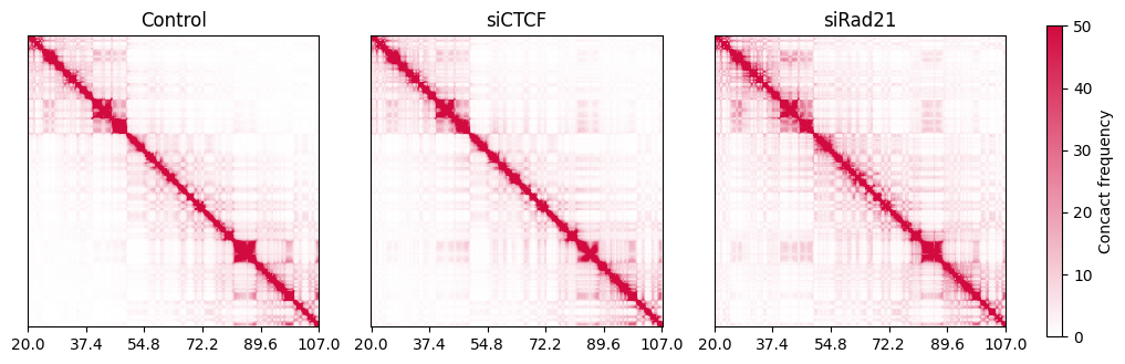
10.1. Chromosome 14, 20 Mbp to 107 Mbp¶

As an example, we plot the contact matrix of the entire chromosome 14 (from 20 Mbp to 107 Mbp) with 100 kbp resolution. This setting is mainly for viewing the compartment structure.

[33]:

# Load contact maps for chromosome 14
chr = "chr14"
resolution = 100000
norm = "SCALE"

samples = get_samples(samplelist, chr, norm, resolution)
nsample = len(samples)

CustardPyResults_Hi-C/Juicer_hg38/Control/Matrix/intrachromosomal/100000/observed.SCALE.chr14.matrix.gz
CustardPyResults_Hi-C/Juicer_hg38/siCTCF/Matrix/intrachromosomal/100000/observed.SCALE.chr14.matrix.gz
CustardPyResults_Hi-C/Juicer_hg38/siRad21/Matrix/intrachromosomal/100000/observed.SCALE.chr14.matrix.gz

[34]:

s = 20000000  # start position
e = 107000000 # end position
vmin = 0  # minimum value of the color scale
vmax = 50 # maximum value of the color scale

plt.figure(figsize=(10, 5))
for i, sample in enumerate(samples):
    label = samplelist[i]
    ax = plt.subplot(1, 3, i+1)
    mat = sample.getmatrix().loc[s:e,s:e]
    im = ax.imshow(mat, clim=(vmin, vmax), cmap=generate_cmap(['#FFFFFF', '#d10a3f']))
    ax.set_title(label)
    pltxticks_subplot2grid(0, mat.shape[1], s, e, 5, ax=ax)
    ax.set_yticks([])
plt.tight_layout()

cbar = plt.colorbar(im, ax=plt.gcf().axes, orientation='vertical', fraction=0.015, pad=0.04)
cbar.set_label('Concact frequency')

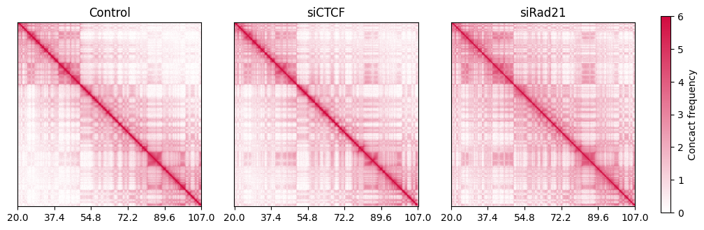
../_images/content_CustardPy_API_7_0.png

Alternatively, you can use the log scale contact frequency with the getlog function to emphasize the TAD and compartment structure.

[35]:

s = 20000000  # start position
e = 107000000 # end position
vmin = 0  # minimum value of the color scale
vmax = 6 # maximum value of the color scale

plt.figure(figsize=(10, 5))
for i, sample in enumerate(samples):
    label = samplelist[i]
    ax = plt.subplot(1, 3, i+1)
    mat = sample.getlog().loc[s:e,s:e]
    im = ax.imshow(mat, clim=(vmin, vmax), cmap=generate_cmap(['#FFFFFF', '#d10a3f']))
    ax.set_title(label)
    pltxticks_subplot2grid(0, mat.shape[1], s, e, 5, ax=ax)
    ax.set_yticks([])
plt.tight_layout()

cbar = plt.colorbar(im, ax=plt.gcf().axes, orientation='vertical', fraction=0.015, pad=0.04)
cbar.set_label('Concact frequency')

../_images/content_CustardPy_API_9_0.png

10.2. chromosome 21, 25 Mbp to 31 Mbp¶

Next, we plot the region from 25 Mbp to 31 Mbp of chromosome 21 at 25 kbp resolution. This region corresponds to the Figure 1A of [Haarhuis et al. Cell, 2017].

[36]:

resolution = 25000
norm = "SCALE"
chr="chr21"

samples = get_samples(samplelist, chr, norm, resolution)
nsample = len(samples)

CustardPyResults_Hi-C/Juicer_hg38/Control/Matrix/intrachromosomal/25000/observed.SCALE.chr21.matrix.gz
CustardPyResults_Hi-C/Juicer_hg38/siCTCF/Matrix/intrachromosomal/25000/observed.SCALE.chr21.matrix.gz
CustardPyResults_Hi-C/Juicer_hg38/siRad21/Matrix/intrachromosomal/25000/observed.SCALE.chr21.matrix.gz

[37]:

s = 25000000
e = 31000000
vmax = 100
vmin = 0

plt.figure(figsize=(12, 10))
for i, sample in enumerate(samples):
    label = samplelist[i]
    ax = plt.subplot(1, 3, i+1)
    mat = sample.getmatrix().loc[s:e,s:e]
    im = ax.imshow(mat, clim=(vmin, vmax), cmap=generate_cmap(['#FFFFFF', '#d10a3f']))
    ax.set_title(label)
    pltxticks_subplot2grid(0, mat.shape[1], s, e, 5, ax=ax)
    ax.set_yticks([])
plt.tight_layout()

cbar = plt.colorbar(im, ax=plt.gcf().axes, orientation='vertical', fraction=0.015, pad=0.04)
cbar.set_label('Concact frequency')

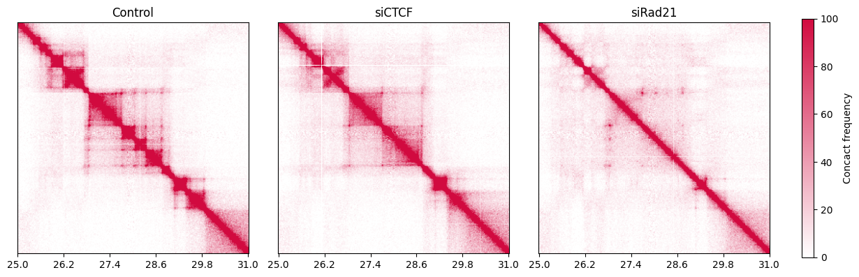
../_images/content_CustardPy_API_12_0.png

The heatmaps clearly show the difference in TAD and loop structures between samples.

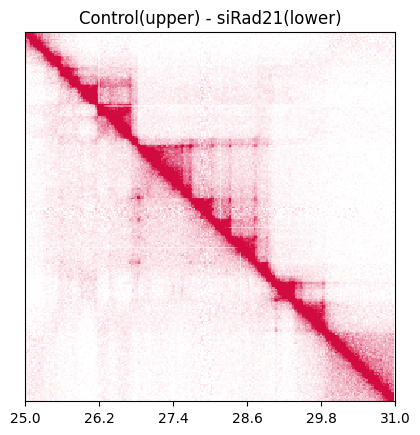
10.3. Plotting a sample pair in a single heatmap¶

Use the plot_SamplePair_triu function to plot a sample pair in a single heatmap. Here we visualize Control and siRad21.

[38]:

resolution=25000
s = 25000000
e = 31000000
vmax = 100
vmin = 0

sample1 = samples[0]
sample2 = samples[2]
label1 = samplelist[0]
label2 = samplelist[2]

plot_SamplePair_triu(sample1, sample2, label1, label2,
                     resolution, s, e, vmax, vmin)

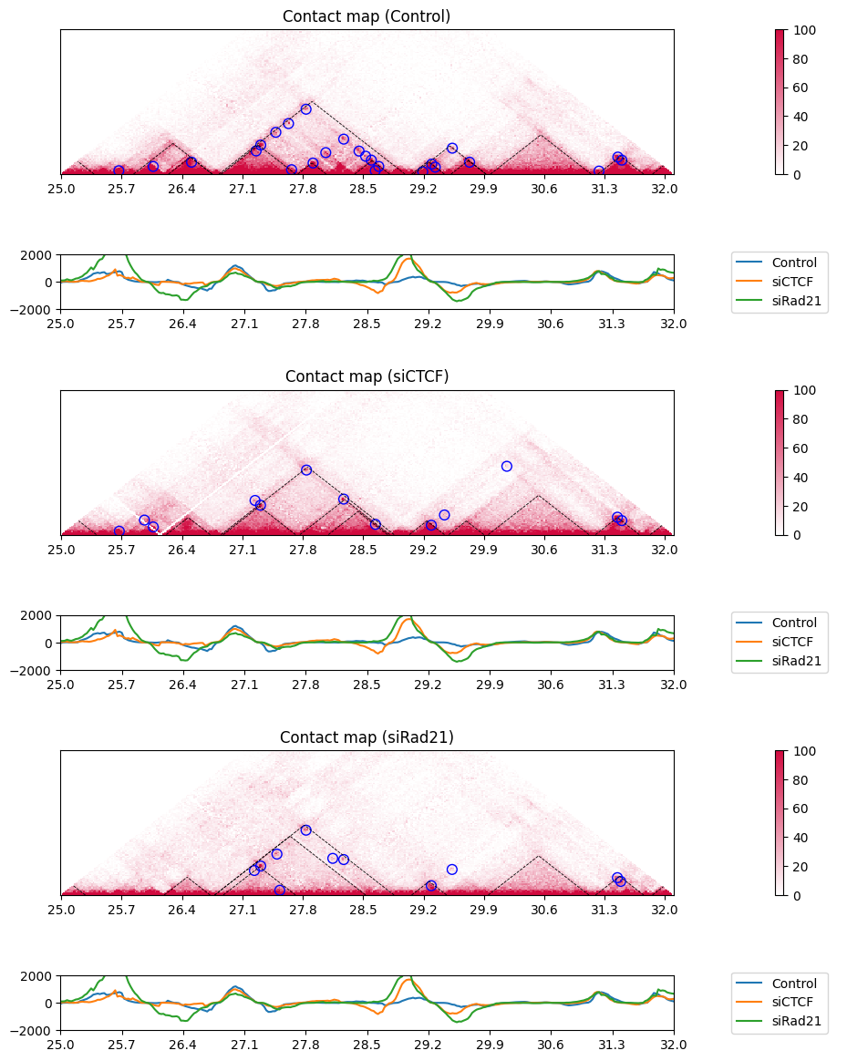
../_images/content_CustardPy_API_15_0.png

10.4. Triangle heatmap with TADs and loops¶

Let’s visualize triangle heatmaps. CustardPy has a plot_HiC_Map function to visualize the Hi-C triangle heatmap.

Here we also visualize TADs and loops by specifying the path of the TADs and the loops called in the CustardPy workflow (see the tutorial for details). The loaded file paths are displayed in the logs, so you can verify that the correct files are being visualized.

[39]:

chr="chr21"
s = 25000000
e = 31000000
resolution = 25000
norm = "SCALE"

# Parameters for drawing
nrow_now = 0
nrow_heatmap = 4
nrow = nrow_heatmap * 3
colspan_plot = 12
colspan_colorbar = 2
colspan_full = (colspan_plot + colspan_colorbar)
vmax = 100  # maximum value of the color scale
vmin = 0    # minimum value of the color scale
distancemax = 0

plt.figure(figsize=(8, 8))
for i, sample in enumerate(samples):
    label = samplelist[i]
    tadfile = "CustardPyResults_Hi-C/Juicer_hg38/" + label + "/TAD/" + norm + "/" + str(resolution) + "_blocks.bedpe"
    loopfile = "CustardPyResults_Hi-C/Juicer_hg38/" + label + "/loops/" + norm + "/merged_loops.bedpe"

    plot_HiC_Map(nrow, nrow_now, nrow_heatmap, sample, label, chr,
                type, resolution, vmax, vmin, s, e, distancemax,
                colspan_plot, colspan_colorbar, colspan_full,
                tadfile=tadfile, loopfile=loopfile)
    nrow_now += nrow_heatmap

plt.tight_layout()

CustardPyResults_Hi-C/Juicer_hg38/Control/TAD/SCALE/25000_blocks.bedpe
CustardPyResults_Hi-C/Juicer_hg38/Control/loops/SCALE/merged_loops.bedpe
CustardPyResults_Hi-C/Juicer_hg38/siCTCF/TAD/SCALE/25000_blocks.bedpe
CustardPyResults_Hi-C/Juicer_hg38/siCTCF/loops/SCALE/merged_loops.bedpe
CustardPyResults_Hi-C/Juicer_hg38/siRad21/TAD/SCALE/25000_blocks.bedpe
CustardPyResults_Hi-C/Juicer_hg38/siRad21/loops/SCALE/merged_loops.bedpe

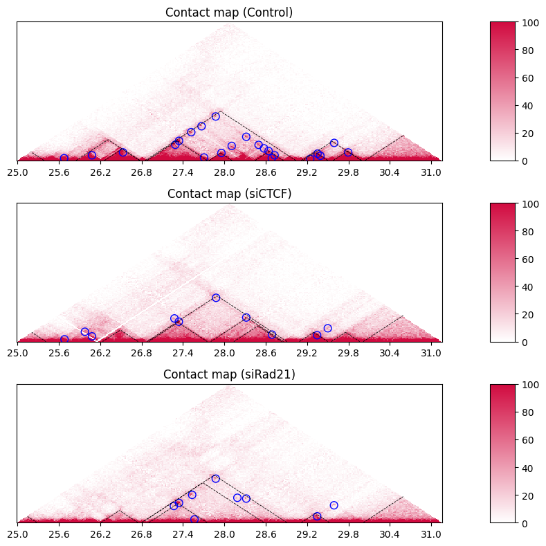
../_images/content_CustardPy_API_17_1.png

The black dashed lines and blue circles indicate TADs and loops, respectively.

If you don’t want to plot TADs and loops, simply skip loading them.

[40]:

chr="chr21"
s = 25000000
e = 31000000
resolution = 25000
norm = "SCALE"

# Parameters for drawing
nrow_now = 0
nrow_heatmap = 4
nrow = nrow_heatmap * 3
colspan_plot = 12
colspan_colorbar = 2
colspan_full = (colspan_plot + colspan_colorbar)
vmax = 100  # maximum value of the color scale
vmin = 0    # minimum value of the color scale
distancemax = 0

plt.figure(figsize=(8, 8))
for i, sample in enumerate(samples):
    label = samplelist[i]
    plot_HiC_Map(nrow, nrow_now, nrow_heatmap, sample, label, chr,
                type, resolution, vmax, vmin, s, e, distancemax,
                colspan_plot, colspan_colorbar, colspan_full)
    nrow_now += nrow_heatmap

plt.tight_layout()

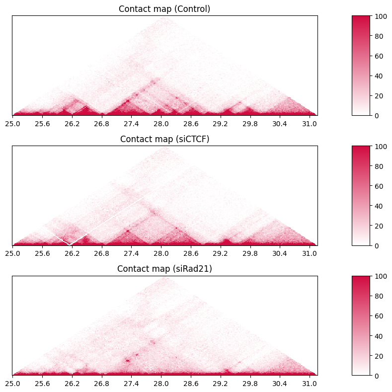
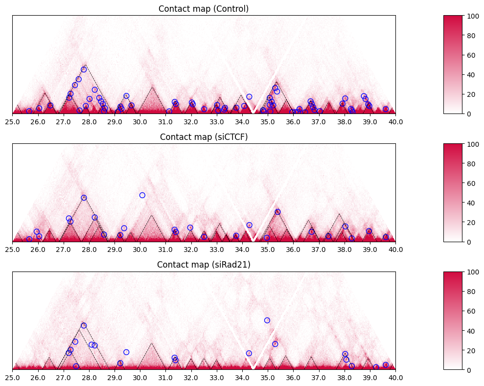
../_images/content_CustardPy_API_19_0.png

When visualizing a broader region, the triangle becomes too large to see each TAD and loop. In this case, set the distance_max parameter in the drawHeatmapTriangle_subplot2grid function to limit the maximum distance of the triangles.

[41]:

chr="chr21"
s = 25000000
e = 40000000
resolution = 25000
norm = "SCALE"
distancemax = 3000000 # Maximum distance for visualization

# Parameters for drawing
nrow_now = 0
nrow_heatmap = 4
nrow = nrow_heatmap * 3
colspan_plot = 12
colspan_colorbar = 2
colspan_full = (colspan_plot + colspan_colorbar)
vmax = 100  # maximum value of the color scale
vmin = 0    # minimum value of the color scale

plt.figure(figsize=(10, 8))
for i, sample in enumerate(samples):
    label = samplelist[i]
    tadfile = "CustardPyResults_Hi-C/Juicer_hg38/" + label + "/TAD/" + norm + "/" + str(resolution) + "_blocks.bedpe"
    loopfile = "CustardPyResults_Hi-C/Juicer_hg38/" + label + "/loops/" + norm + "/merged_loops.bedpe"

    plot_HiC_Map(nrow, nrow_now, nrow_heatmap, sample, label, chr,
                type, resolution, vmax, vmin, s, e, distancemax,
                colspan_plot, colspan_colorbar, colspan_full,
                tadfile=tadfile, loopfile=loopfile)
    nrow_now += nrow_heatmap

plt.tight_layout()

CustardPyResults_Hi-C/Juicer_hg38/Control/TAD/SCALE/25000_blocks.bedpe
CustardPyResults_Hi-C/Juicer_hg38/Control/loops/SCALE/merged_loops.bedpe
CustardPyResults_Hi-C/Juicer_hg38/siCTCF/TAD/SCALE/25000_blocks.bedpe
CustardPyResults_Hi-C/Juicer_hg38/siCTCF/loops/SCALE/merged_loops.bedpe
CustardPyResults_Hi-C/Juicer_hg38/siRad21/TAD/SCALE/25000_blocks.bedpe
CustardPyResults_Hi-C/Juicer_hg38/siRad21/loops/SCALE/merged_loops.bedpe

../_images/content_CustardPy_API_21_1.png

10.4.1. Adding 3D Features¶

Here is the way to visualize some 3D features.

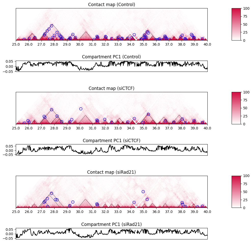
10.5. Compartment PC1¶

To distinguish the genomic positions from bin positions, let’s define figstart/figend and sbin/ebin. The resolution is 25 kbp.

[42]:

figstart = 25000000
figend = 40000000
resolution = 25000
sbin = int(figstart / resolution)
ebin = int(figend   / resolution)

The plot_PC1 function plots the compartment PC1. The positive and negative values indicate the compartments A and B, respectively.

[43]:

norm = "SCALE"

nrow_heatmap = 4
nrow_eigen = 2
nrow = (nrow_heatmap +1 + nrow_eigen +1) *3
nrow_now = 0
colspan_plot = 12
colspan_colorbar = 2
colspan_full = (colspan_plot + colspan_colorbar)
vmax = 100
vmin = 0

plt.figure(figsize=(10, 10))
for i, sample in enumerate(samples):
    label = samplelist[i]
    tadfile = "CustardPyResults_Hi-C/Juicer_hg38/" + label + "/TAD/" + norm + "/" + str(resolution) + "_blocks.bedpe"
    loopfile = "CustardPyResults_Hi-C/Juicer_hg38/" + label + "/loops/" + norm + "/merged_loops.bedpe"

    plot_HiC_Map(nrow, nrow_now, nrow_heatmap, sample, label, chr,
                type, resolution, vmax, vmin, s, e, distancemax,
                colspan_plot, colspan_colorbar, colspan_full,
                tadfile=tadfile, loopfile=loopfile)
    nrow_now += nrow_heatmap + 1

    plot_PC1(nrow, nrow_now, nrow_eigen, sample, label, sbin, ebin, colspan_plot, colspan_full)
    nrow_now += nrow_eigen + 1

plt.tight_layout()

CustardPyResults_Hi-C/Juicer_hg38/Control/TAD/SCALE/25000_blocks.bedpe
CustardPyResults_Hi-C/Juicer_hg38/Control/loops/SCALE/merged_loops.bedpe
CustardPyResults_Hi-C/Juicer_hg38/siCTCF/TAD/SCALE/25000_blocks.bedpe
CustardPyResults_Hi-C/Juicer_hg38/siCTCF/loops/SCALE/merged_loops.bedpe
CustardPyResults_Hi-C/Juicer_hg38/siRad21/TAD/SCALE/25000_blocks.bedpe
CustardPyResults_Hi-C/Juicer_hg38/siRad21/loops/SCALE/merged_loops.bedpe

../_images/content_CustardPy_API_25_1.png

10.6. Single insulation score¶

[44]:

figstart = 25000000
figend = 32000000
resolution = 25000
sbin = int(figstart / resolution)
ebin = int(figend   / resolution)
distancemax = 3000000 # Maximum distance for visualization
norm = "SCALE"

nrow_heatmap = 4
nrow_feature = 2
nrow = (nrow_heatmap +1 + nrow_feature + 1) * 3
nrow_now = 0
colspan_plot = 12
colspan_colorbar = 1
colspan_legend = 3
colspan_full = (colspan_plot + colspan_colorbar + colspan_legend)
vmax = 100
vmin = 0

plt.figure(figsize=(10, 12))
for i, sample in enumerate(samples):
    label = samplelist[i]
    tadfile = "CustardPyResults_Hi-C/Juicer_hg38/" + label + "/TAD/" + norm + "/" + str(resolution) + "_blocks.bedpe"
    loopfile = "CustardPyResults_Hi-C/Juicer_hg38/" + label + "/loops/" + norm + "/merged_loops.bedpe"

    plot_HiC_Map(nrow, nrow_now, nrow_heatmap, sample, label, chr,
                type, resolution, vmax, vmin, s, e, distancemax,
                colspan_plot, colspan_colorbar, colspan_full,
                tadfile=tadfile, loopfile=loopfile)
    nrow_now += nrow_heatmap + 1

    plot_single_insulation_score(sample, label, nrow, nrow_now, nrow_feature,
                                 figstart, figend, sbin, ebin,
                                 colspan_plot, colspan_colorbar, colspan_legend, colspan_full)

    nrow_now += nrow_feature + 1

plt.tight_layout()

CustardPyResults_Hi-C/Juicer_hg38/Control/TAD/SCALE/25000_blocks.bedpe
CustardPyResults_Hi-C/Juicer_hg38/Control/loops/SCALE/merged_loops.bedpe
CustardPyResults_Hi-C/Juicer_hg38/siCTCF/TAD/SCALE/25000_blocks.bedpe
CustardPyResults_Hi-C/Juicer_hg38/siCTCF/loops/SCALE/merged_loops.bedpe
CustardPyResults_Hi-C/Juicer_hg38/siRad21/TAD/SCALE/25000_blocks.bedpe
CustardPyResults_Hi-C/Juicer_hg38/siRad21/loops/SCALE/merged_loops.bedpe

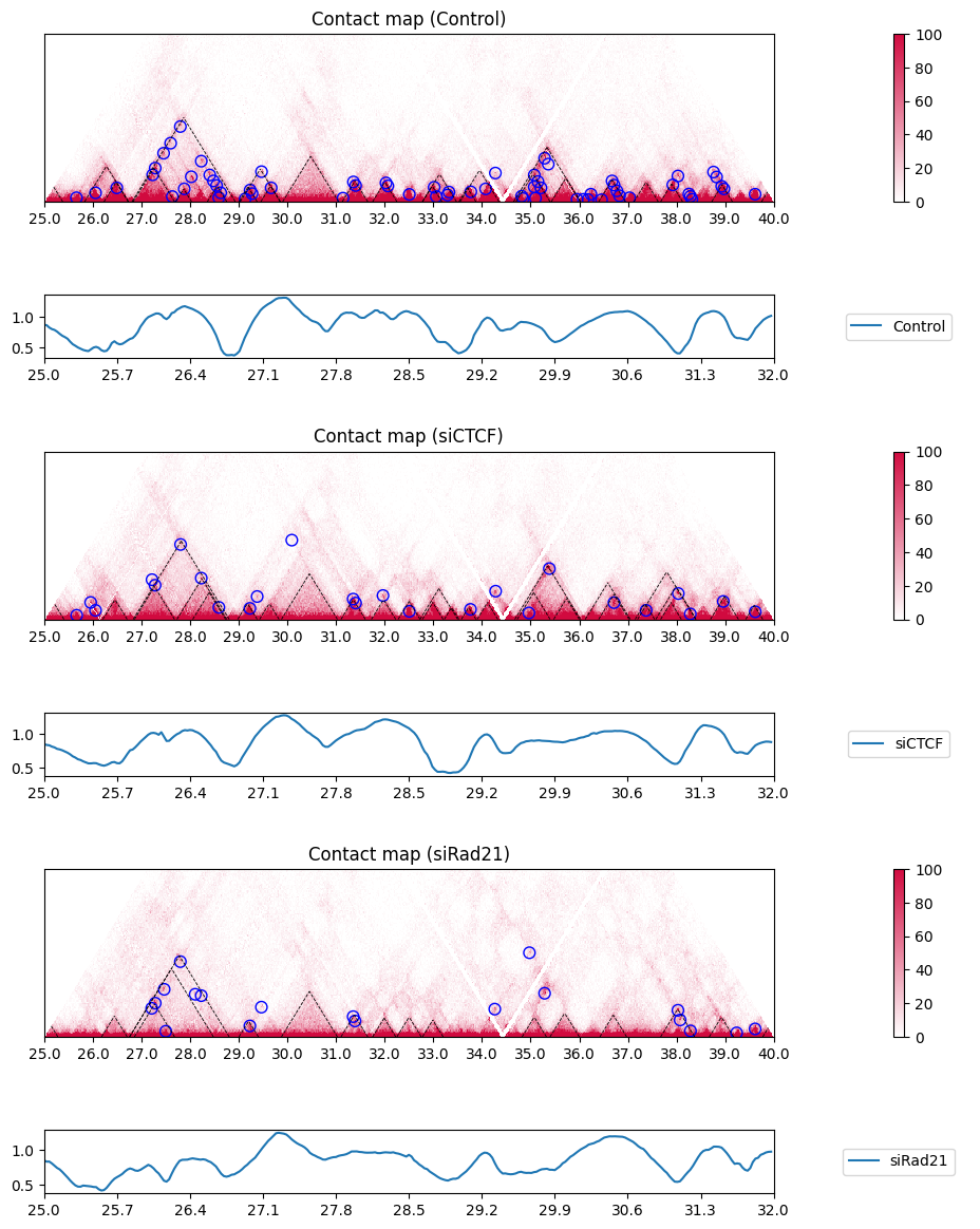
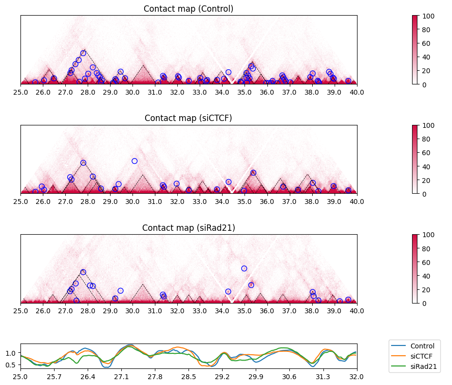
../_images/content_CustardPy_API_27_1.png

You can view the insulation scores of all samples in this way:

[45]:

figstart = 25000000
figend = 32000000
resolution = 25000
sbin = int(figstart / resolution)
ebin = int(figend   / resolution)
distancemax = 3000000 # Maximum distance for visualization
norm = "SCALE"

nrow_heatmap = 4
nrow_feature = 2
nrow = (nrow_heatmap +1) * 3 + nrow_feature
nrow_now = 0
colspan_plot = 12
colspan_colorbar = 1
colspan_legend = 3
colspan_full = (colspan_plot + colspan_colorbar + colspan_legend)
vmax = 100
vmin = 0

plt.figure(figsize=(10, 8))
for i, sample in enumerate(samples):
    label = samplelist[i]
    tadfile = "CustardPyResults_Hi-C/Juicer_hg38/" + label + "/TAD/" + norm + "/" + str(resolution) + "_blocks.bedpe"
    loopfile = "CustardPyResults_Hi-C/Juicer_hg38/" + label + "/loops/" + norm + "/merged_loops.bedpe"

    plot_HiC_Map(nrow, nrow_now, nrow_heatmap, sample, label, chr,
                type, resolution, vmax, vmin, s, e, distancemax,
                colspan_plot, colspan_colorbar, colspan_full,
                tadfile=tadfile, loopfile=loopfile)
    nrow_now += nrow_heatmap +1

plot_single_insulation_score(samples, samplelist, nrow, nrow_now, nrow_feature,
                             figstart, figend, sbin, ebin,
                             colspan_plot, colspan_colorbar, colspan_legend, colspan_full)

plt.tight_layout()

CustardPyResults_Hi-C/Juicer_hg38/Control/TAD/SCALE/25000_blocks.bedpe
CustardPyResults_Hi-C/Juicer_hg38/Control/loops/SCALE/merged_loops.bedpe
CustardPyResults_Hi-C/Juicer_hg38/siCTCF/TAD/SCALE/25000_blocks.bedpe
CustardPyResults_Hi-C/Juicer_hg38/siCTCF/loops/SCALE/merged_loops.bedpe
CustardPyResults_Hi-C/Juicer_hg38/siRad21/TAD/SCALE/25000_blocks.bedpe
CustardPyResults_Hi-C/Juicer_hg38/siRad21/loops/SCALE/merged_loops.bedpe

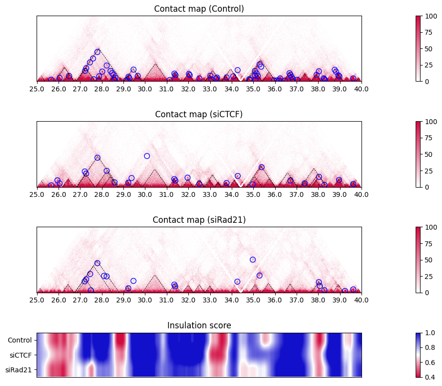
../_images/content_CustardPy_API_29_1.png

If you want to display the insulation score of the samples as a heatmap, use the options heatmap=True, lineplot=False. In the heatmap, red regions indicate lower values (i.e. insulated regions).

[46]:

figstart = 25000000
figend = 32000000
resolution = 25000
sbin = int(figstart / resolution)
ebin = int(figend   / resolution)
distancemax = 3000000 # Maximum distance for visualization
norm = "SCALE"

nrow_heatmap = 4
nrow_feature = 3
nrow = (nrow_heatmap +1) * 3 + nrow_feature
nrow_now = 0
colspan_plot = 12
colspan_colorbar = 1
colspan_legend = 3
colspan_full = (colspan_plot + colspan_colorbar + colspan_legend)
vmax = 100
vmin = 0

plt.figure(figsize=(10, 8))
for i, sample in enumerate(samples):
    label = samplelist[i]
    tadfile = "CustardPyResults_Hi-C/Juicer_hg38/" + label + "/TAD/" + norm + "/" + str(resolution) + "_blocks.bedpe"
    loopfile = "CustardPyResults_Hi-C/Juicer_hg38/" + label + "/loops/" + norm + "/merged_loops.bedpe"

    plot_HiC_Map(nrow, nrow_now, nrow_heatmap, sample, label, chr,
                type, resolution, vmax, vmin, s, e, distancemax,
                colspan_plot, colspan_colorbar, colspan_full,
                tadfile=tadfile, loopfile=loopfile)
    nrow_now += nrow_heatmap +1

plot_single_insulation_score(samples, samplelist, nrow, nrow_now, nrow_feature,
                             figstart, figend, sbin, ebin,
                             colspan_plot, colspan_colorbar, colspan_legend, colspan_full,
                             heatmap=True, lineplot=False)

plt.tight_layout()

CustardPyResults_Hi-C/Juicer_hg38/Control/TAD/SCALE/25000_blocks.bedpe
CustardPyResults_Hi-C/Juicer_hg38/Control/loops/SCALE/merged_loops.bedpe
CustardPyResults_Hi-C/Juicer_hg38/siCTCF/TAD/SCALE/25000_blocks.bedpe
CustardPyResults_Hi-C/Juicer_hg38/siCTCF/loops/SCALE/merged_loops.bedpe
CustardPyResults_Hi-C/Juicer_hg38/siRad21/TAD/SCALE/25000_blocks.bedpe
CustardPyResults_Hi-C/Juicer_hg38/siRad21/loops/SCALE/merged_loops.bedpe

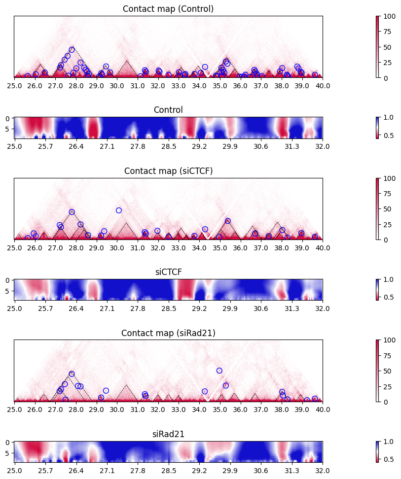
../_images/content_CustardPy_API_31_1.png

10.7. Multi-scale insulation scores¶

The plot_multi_insulation_score function plots multi-scale insulation scores. The plot is similar to the one above (single insulation score for multiple samples), but note that this heatmap shows the insulation score at the different scale for each sample.

[47]:

figstart = 25000000
figend = 32000000
resolution = 25000
sbin = int(figstart / resolution)
ebin = int(figend   / resolution)
distancemax = 3000000 # Maximum distance for visualization
norm = "SCALE"

nrow_heatmap = 4
nrow_feature = 2
nrow = (nrow_heatmap +1 + nrow_feature + 1) * 3
nrow_now = 0
colspan_plot = 12
colspan_colorbar = 1
colspan_legend = 3
colspan_full = (colspan_plot + colspan_colorbar + colspan_legend)
vmax = 100
vmin = 0

plt.figure(figsize=(9, 10))
for i, sample in enumerate(samples):
    label = samplelist[i]
    tadfile = "CustardPyResults_Hi-C/Juicer_hg38/" + label + "/TAD/" + norm + "/" + str(resolution) + "_blocks.bedpe"
    loopfile = "CustardPyResults_Hi-C/Juicer_hg38/" + label + "/loops/" + norm + "/merged_loops.bedpe"

    plot_HiC_Map(nrow, nrow_now, nrow_heatmap, sample, label, chr,
                type, resolution, vmax, vmin, s, e, distancemax,
                colspan_plot, colspan_colorbar, colspan_full,
                tadfile=tadfile, loopfile=loopfile)
    nrow_now += nrow_heatmap + 1

    plot_multi_insulation_score(sample, label, nrow, nrow_now, nrow_feature,
                                figstart, figend, sbin, ebin,
                                colspan_plot, colspan_colorbar, colspan_full)
    nrow_now += nrow_feature + 1

plt.tight_layout()

CustardPyResults_Hi-C/Juicer_hg38/Control/TAD/SCALE/25000_blocks.bedpe
CustardPyResults_Hi-C/Juicer_hg38/Control/loops/SCALE/merged_loops.bedpe
CustardPyResults_Hi-C/Juicer_hg38/siCTCF/TAD/SCALE/25000_blocks.bedpe
CustardPyResults_Hi-C/Juicer_hg38/siCTCF/loops/SCALE/merged_loops.bedpe
CustardPyResults_Hi-C/Juicer_hg38/siRad21/TAD/SCALE/25000_blocks.bedpe
CustardPyResults_Hi-C/Juicer_hg38/siRad21/loops/SCALE/merged_loops.bedpe

../_images/content_CustardPy_API_33_1.png

10.8. Directionality index¶

Use the plot_directionality_index function to plot the directionality index.

[48]:

figstart = 25000000
figend = 32000000
resolution = 25000
sbin = int(figstart / resolution)
ebin = int(figend   / resolution)
distance = 500000 # distance for DI
distancemax = 3000000 # Maximum distance for visualization
norm = "SCALE"

nrow_heatmap = 4
nrow_feature = 2
nrow = (nrow_heatmap +1 + nrow_feature + 1) * 3
nrow_now = 0
colspan_plot = 12
colspan_colorbar = 1
colspan_legend = 3
colspan_full = (colspan_plot + colspan_colorbar + colspan_legend)
vmax = 100
vmin = 0
DI_vmin = -2000  # Mimnimum value of Directionality index
DI_vmax = 2000   # Maximum value of Directionality index

plt.figure(figsize=(10, 12))
for i, sample in enumerate(samples):
    label = samplelist[i]
    tadfile = "CustardPyResults_Hi-C/Juicer_hg38/" + label + "/TAD/" + norm + "/" + str(resolution) + "_blocks.bedpe"
    loopfile = "CustardPyResults_Hi-C/Juicer_hg38/" + label + "/loops/" + norm + "/merged_loops.bedpe"

    plot_HiC_Map(nrow, nrow_now, nrow_heatmap, sample, label, chr,
                type, resolution, vmax, vmin, figstart, figend, distancemax,
                colspan_plot, colspan_colorbar, colspan_full,
                tadfile=tadfile, loopfile=loopfile)
    nrow_now += nrow_heatmap + 1

    plot_directionality_index(samples, samplelist, nrow, nrow_now, nrow_feature,
                              sbin, ebin, figstart, figend, distance,
                              colspan_plot, colspan_colorbar, colspan_legend, colspan_full,
                              vmin=DI_vmin, vmax=DI_vmax)
    nrow_now += nrow_feature + 1

plt.tight_layout()

CustardPyResults_Hi-C/Juicer_hg38/Control/TAD/SCALE/25000_blocks.bedpe
CustardPyResults_Hi-C/Juicer_hg38/Control/loops/SCALE/merged_loops.bedpe
CustardPyResults_Hi-C/Juicer_hg38/siCTCF/TAD/SCALE/25000_blocks.bedpe
CustardPyResults_Hi-C/Juicer_hg38/siCTCF/loops/SCALE/merged_loops.bedpe
CustardPyResults_Hi-C/Juicer_hg38/siRad21/TAD/SCALE/25000_blocks.bedpe
CustardPyResults_Hi-C/Juicer_hg38/siRad21/loops/SCALE/merged_loops.bedpe

../_images/content_CustardPy_API_35_1.png

[49]:

figstart = 25000000
figend = 32000000
resolution = 25000
sbin = int(figstart / resolution)
ebin = int(figend   / resolution)
distance = 500000 # distance for DI
distancemax = 3000000 # Maximum distance for visualization
norm = "SCALE"

nrow_heatmap = 4
nrow_feature = 3
nrow = (nrow_heatmap +1) * 3 + nrow_feature
nrow_now = 0
colspan_plot = 12
colspan_colorbar = 1
colspan_legend = 1
colspan_full = (colspan_plot + colspan_colorbar + colspan_legend)
vmax = 100
vmin = 0

plt.figure(figsize=(10, 8))
for i, sample in enumerate(samples):
    label = samplelist[i]
    tadfile = "CustardPyResults_Hi-C/Juicer_hg38/" + label + "/TAD/" + norm + "/" + str(resolution) + "_blocks.bedpe"
    loopfile = "CustardPyResults_Hi-C/Juicer_hg38/" + label + "/loops/" + norm + "/merged_loops.bedpe"

    plot_HiC_Map(nrow, nrow_now, nrow_heatmap, sample, label, chr,
                type, resolution, vmax, vmin, s, e, distancemax,
                colspan_plot, colspan_colorbar, colspan_full,
                tadfile=tadfile, loopfile=loopfile)
    nrow_now += nrow_heatmap +1

plot_directionality_index(samples, samplelist, nrow, nrow_now, nrow_feature,
                          sbin, ebin, figstart, figend, distance,
                          colspan_plot, colspan_colorbar, colspan_legend, colspan_full,
                          vmin=DI_vmin, vmax=DI_vmax, heatmap=True, lineplot=False)

plt.tight_layout()

CustardPyResults_Hi-C/Juicer_hg38/Control/TAD/SCALE/25000_blocks.bedpe
CustardPyResults_Hi-C/Juicer_hg38/Control/loops/SCALE/merged_loops.bedpe
CustardPyResults_Hi-C/Juicer_hg38/siCTCF/TAD/SCALE/25000_blocks.bedpe
CustardPyResults_Hi-C/Juicer_hg38/siCTCF/loops/SCALE/merged_loops.bedpe
CustardPyResults_Hi-C/Juicer_hg38/siRad21/TAD/SCALE/25000_blocks.bedpe
CustardPyResults_Hi-C/Juicer_hg38/siRad21/loops/SCALE/merged_loops.bedpe

../_images/content_CustardPy_API_36_1.png

10.8.1. Log ratio heatmap¶

To directly examine the depletion effect in the contact matrix, we visualize the log ratio heatmap here. First, create log-ratio matrix using the make3dmatrixRatio function. The smooth_median_filter parameter is used to smooth the data to mitigate the low coverage of the sparse matrix.

[50]:

smooth_median_filter = 3
Combined = make3dmatrixRatio(samples, smooth_median_filter)
labels = ["siCTCF", "siRad21"]

The Combined object stores the log-ratio matrix of siCTCF/Control and siRad21/Control. You can use it to view the log-ratio heatmap as shown below.

[51]:

figstart = 27500000
figend   = 32500000
resolution = 25000
sbin = int(figstart / resolution)
ebin = int(figend   / resolution)
vmax = 1
vmin = -1

plt.figure(figsize=(6, 3))
for i in range(len(labels)):
    ax = plt.subplot(1, 2, i+1)
    im = ax.imshow(Combined[i, sbin:ebin,sbin:ebin], clim=(vmin, vmax), cmap=cm)
    ax.set_title(labels[i])
    pltxticks_subplot2grid(0, ebin-sbin, figstart, figend, 5, ax=ax)
    ax.set_yticks([])

plt.tight_layout()
cbar = plt.colorbar(im, ax=plt.gcf().axes, orientation='vertical', fraction=0.015, pad=0.04)
cbar.set_label('log enrichment')

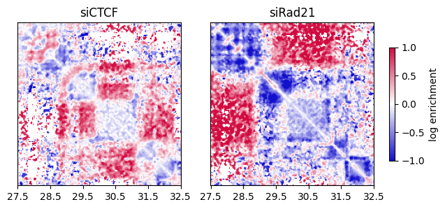
../_images/content_CustardPy_API_40_0.png

Red and blue regions indicate increased and decreased contact frequency, respectively, after depletion.

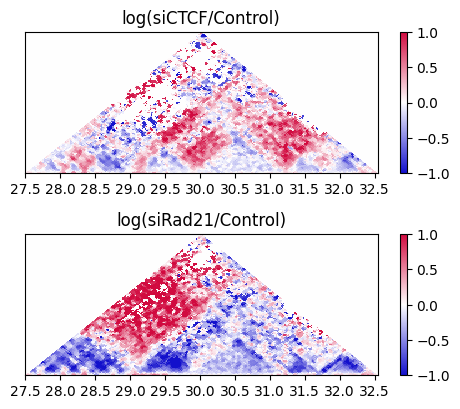
To draw the triangle heatmap, use the drawHeatmapTriangle_subplot2grid function.

[52]:

nrow = 8
nrow_now = 0
colspan_full = 30
figstart = 27500000
figend   = 32500000

plt.figure(figsize=(6, 8))
for i, sample in enumerate(Combined):
    ax  = plt.subplot2grid((nrow, colspan_full), (nrow_now, 0), rowspan=2, colspan=24)
    drawHeatmapTriangle_subplot2grid(sample, resolution,
                                     figstart=figstart, figend=figend,
                                     vmax=1, vmin=-1, cmap=cm,
                                     label=labels[i], xticks=True,
                                     logratio=True, control_label='Control')
    nrow_now += 2

plt.tight_layout()

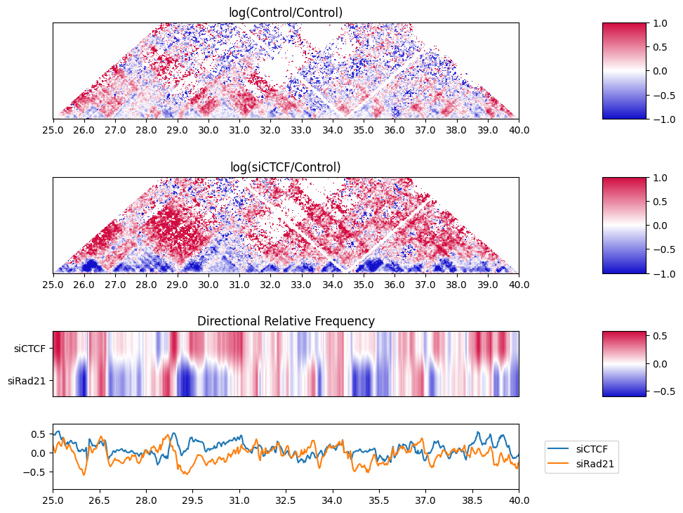
../_images/content_CustardPy_API_42_0.png

10.9. Directional Relative Frequency¶

Recently, we have defined a new score Directional Relative Frequency (DRF) that captures the asymmetric changes in inter-TAD interactions after depletion [Nakato et al, Nat Commun., 2023].

The plot_directional_relative_frequency function visualizes the line plot and heatmap of the DRF.

[53]:

figstart = 25000000
figend = 40000000
resolution = 25000
sbin = int(figstart / resolution)
ebin = int(figend   / resolution)
distancemax = 5000000 # Maximum distance for visualization
norm = "SCALE"

nrow_heatmap = 4
nrow_feature = 3
nrow = (nrow_heatmap +1 + nrow_feature + 1) * 3
nrow_now = 0
colspan_plot = 12
colspan_colorbar = 2
colspan_legend = 2
colspan_full = (colspan_plot + colspan_colorbar + colspan_legend)
vmax = 1
vmin = -1

plt.figure(figsize=(10, 12))
for i, sample in enumerate(Combined):
    label = samplelist[i]
    heatmap_ax  = plt.subplot2grid((nrow, colspan_full), (nrow_now, 0),
                                    rowspan=nrow_heatmap, colspan=colspan_plot)
    colorbar_ax = plt.subplot2grid((nrow, colspan_full), (nrow_now, colspan_plot +1),
                                    rowspan=nrow_heatmap, colspan=colspan_colorbar)

    drawHeatmapTriangle_subplot2grid(sample, resolution, figstart=figstart, figend=figend,
                                     vmax=vmax, vmin=vmin, cmap=cm, label=label, xticks=True,
                                     logratio=True, control_label='Control',
                                     heatmap_ax=heatmap_ax, colorbar_ax=colorbar_ax)
    nrow_now += nrow_heatmap + 1

plot_directional_relative_frequency(samples, samplelist,  nrow, nrow_now, nrow_feature,
                                    sbin, ebin, figstart, figend, resolution,
                                    True, True,
                                    colspan_plot, colspan_colorbar, colspan_legend, colspan_full)

plt.tight_layout()

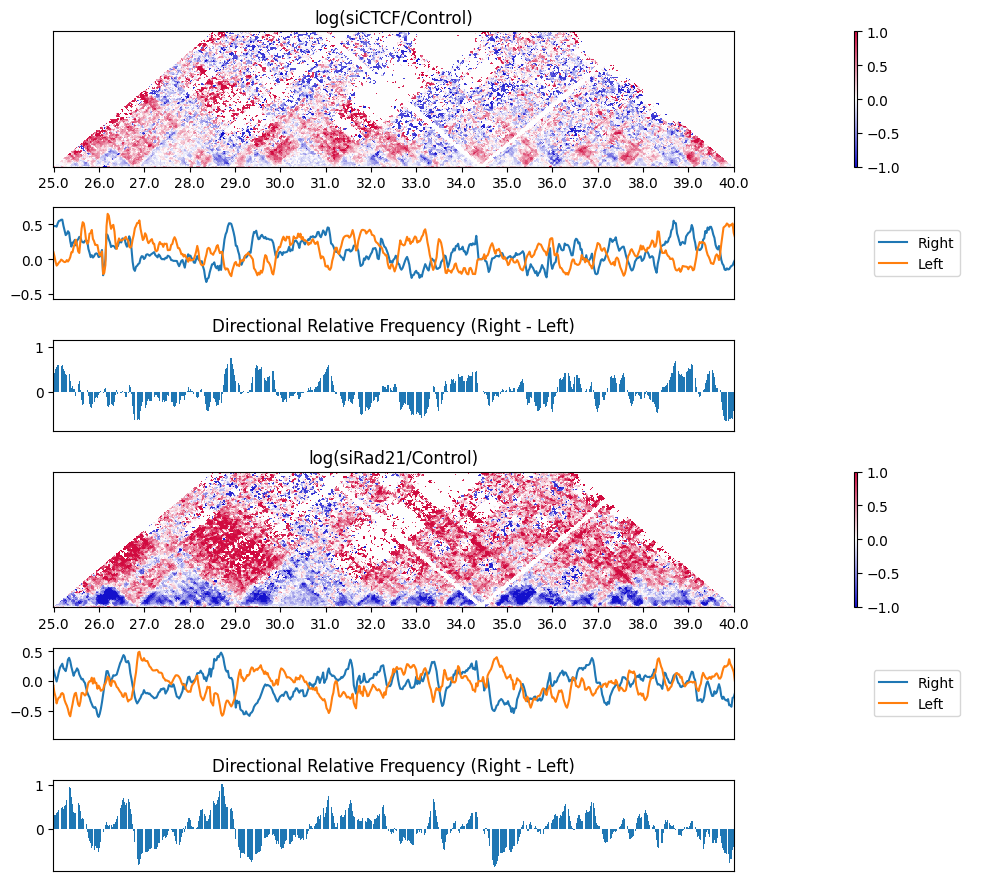
../_images/content_CustardPy_API_44_0.png

The DRF does not distinguish whether the right side is enriched or the left side is depleted when the score is high. By using the plot_triangle_ratio_multi function, it is possible to visualize the scores on both the left and right sides.

[54]:

figstart = 25000000
figend = 40000000
resolution = 25000
sbin = int(figstart / resolution)
ebin = int(figend   / resolution)
distancemax = 5000000 # Maximum distance for visualization

nrow_heatmap = 4
nrow_feature = 3
nrow = (nrow_heatmap +1 + nrow_feature + 1) * 3
nrow_now = 0
colspan_plot = 12
colspan_colorbar = 1
colspan_legend = 3
colspan_full = (colspan_plot + colspan_colorbar + colspan_legend)
vmin = -1
vmax = 1

plt.figure(figsize=(10, 12))
plot_triangle_ratio_multi(samples, samplelist, nrow, nrow_now, nrow_heatmap, nrow_feature,
                                  sbin, ebin, figstart, figend, distancemax, resolution,
                                  vmin, vmax, colspan_plot, colspan_colorbar, colspan_legend, colspan_full)

plt.tight_layout()

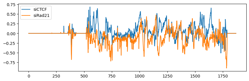
../_images/content_CustardPy_API_46_0.png

To obtain the distribution of the DRF, you can use the get_drf_matrix function.

[55]:

drf_right = True
drf_left = True
DRFMatrix = get_drf_matrix(samples, resolution, drf_right, drf_left)

plt.figure(figsize=(10, 3))
for i, sample in enumerate(DRFMatrix):
   plt.plot(sample, label=labels[i])

plt.legend()

[55]:

<matplotlib.legend.Legend at 0x7f6514989e10>

../_images/content_CustardPy_API_48_1.png

[56]:

import session_info

session_info.show()

[56]:

Click to view session information

-----
custardpy           0.7.1
matplotlib          3.8.3
numpy               1.25.2
pandas              1.5.3
scipy               1.10.1
session_info        1.0.0
sklearn             1.2.2
-----

Click to view modules imported as dependencies

PIL                         10.2.0
anyio                       NA
arrow                       1.3.0
asttokens                   NA
attr                        23.1.0
attrs                       23.1.0
babel                       2.11.0
bottleneck                  1.3.7
brotli                      1.0.9
certifi                     2024.02.02
cffi                        1.16.0
charset_normalizer          2.0.4
colorama                    0.4.6
comm                        0.2.1
cycler                      0.12.1
cython_runtime              NA
dateutil                    2.8.2
debugpy                     1.6.7
decorator                   5.1.1
defusedxml                  0.7.1
exceptiongroup              1.2.0
executing                   0.8.3
fastjsonschema              NA
fqdn                        NA
idna                        3.4
ipykernel                   6.28.0
isoduration                 NA
jedi                        0.18.1
jinja2                      3.1.3
joblib                      1.3.2
json5                       NA
jsonpointer                 2.1
jsonschema                  4.19.2
jsonschema_specifications   NA
jupyter_events              0.8.0
jupyter_server              2.10.0
jupyterlab_server           2.25.1
kiwisolver                  1.4.4
markupsafe                  2.0.1
matplotlib_inline           0.1.6
mpl_toolkits                NA
nbformat                    5.9.2
numexpr                     2.8.7
overrides                   NA
packaging                   23.1
parso                       0.8.3
pexpect                     4.8.0
pkg_resources               NA
platformdirs                3.10.0
prometheus_client           NA
prompt_toolkit              3.0.43
psutil                      5.9.8
ptyprocess                  0.7.0
pure_eval                   0.2.2
pydev_ipython               NA
pydevconsole                NA
pydevd                      2.9.5
pydevd_file_utils           NA
pydevd_plugins              NA
pydevd_tracing              NA
pygments                    2.15.1
pyparsing                   3.0.9
pythonjsonlogger            NA
pytz                        2023.3.post1
referencing                 NA
requests                    2.31.0
rfc3339_validator           0.1.4
rfc3986_validator           0.1.1
rpds                        NA
ruamel                      NA
send2trash                  NA
simplejson                  3.17.6
six                         1.16.0
sniffio                     1.3.0
sphinxcontrib               NA
stack_data                  0.2.0
threadpoolctl               2.2.0
tornado                     6.3.3
traitlets                   5.7.1
typing_extensions           NA
uri_template                NA
urllib3                     2.1.0
wcwidth                     0.2.5
webcolors                   1.13
websocket                   1.7.0
yaml                        6.0.1
zmq                         24.0.1
zoneinfo                    NA
zstandard                   0.19.0

-----
IPython             8.20.0
jupyter_client      8.6.0
jupyter_core        5.5.0
jupyterlab          4.0.11
notebook            7.0.8
-----
Python 3.10.13 | packaged by conda-forge | (main, Dec 23 2023, 15:36:39) [GCC 12.3.0]
Linux-6.2.0-39-generic-x86_64-with-glibc2.35
-----
Session information updated at 2024-03-03 18:43