3. Step-by-Step Workflow of Hi-C Analysis#
Here we show the step-by-step analysis of Hi-C with CustardPy. See also the sample scripts in the tutorial on GitHub.
Note
See the Quickstart section for how to run CustardPy using Docker or Apptainer.`
3.1. (Optional) download the FASTQ files#
Here we use the Hi-C samples of human RPE cells from Nakato et al., Nature Communications, 2023 for the example data.
mkdir -p fastq/siCTCF fastq/siRad21 fastq/Control

# siCTCF
wget -nv --timestamping ftp://ftp.sra.ebi.ac.uk/vol1/fastq/SRR178/013/SRR17870713/SRR17870713_1.fastq.gz -P fastq/siCTCF
wget -nv --timestamping ftp://ftp.sra.ebi.ac.uk/vol1/fastq/SRR178/013/SRR17870713/SRR17870713_2.fastq.gz -P fastq/siCTCF
# Control
wget -nv --timestamping ftp://ftp.sra.ebi.ac.uk/vol1/fastq/SRR178/018/SRR17870718/SRR17870718_1.fastq.gz -P fastq/Control
wget -nv --timestamping ftp://ftp.sra.ebi.ac.uk/vol1/fastq/SRR178/018/SRR17870718/SRR17870718_2.fastq.gz -P fastq/Control
# siRad21
wget -nv --timestamping ftp://ftp.sra.ebi.ac.uk/vol1/fastq/SRR178/040/SRR17870740/SRR17870740_1.fastq.gz -P fastq/siRad21
wget -nv --timestamping ftp://ftp.sra.ebi.ac.uk/vol1/fastq/SRR178/040/SRR17870740/SRR17870740_2.fastq.gz -P fastq/siRad21
Check the files are properly downloaded.
$ ls fastq/*
fastq/Control:
SRR17870718_1.fastq.gz  SRR17870718_2.fastq.gz

fastq/siCTCF:
SRR17870713_1.fastq.gz  SRR17870713_2.fastq.gz

fastq/siRad21:
SRR17870740_1.fastq.gz  SRR17870740_2.fastq.gz
3.2. Download the reference genome and build genome index#
For this tutorial, we provide a script gethg38genome.sh in CustardPy that downloads the sequence of human genome build hg38.
# download genome
gethg38genome.sh

# build BWA index
indexdir=bwa-indexes
mkdir -p $indexdir
bwa index -p $indexdir/hg38 genome.hg38.fa
ln -rsf genome.hg38.fa $indexdir/hg38
3.3. Map reads and generate the .hic file#
Using the FASTQ files and the BWA index, juicer_map.sh command generates the .hic file.
build=hg38
gt=genometable.$build.txt
bwaindex=bwa-indexes/$build
fastq_post="_"  # "_" or "_R"
enzyme=MboI
ncore=32

cell=Control # (siCTCF siRad21 as well)
fqdir=fastq/$cell   # FASTQ directory
odir=CustardPyResults_Hi-C/Juicer_$build/$cell  # Output directory

juicer_map.sh -p $ncore $fqdir $odir $build $gt $bwaindex $enzyme $fastq_post
Note
If the number of sequenced reads is extremely large (e.g. GM12878 cells from Rao et al. 2014), the generation of the .hic file will fail with an error due to lack of memory. In such a case, supply the -L option to juicer_map.sh, which allocates a larger amount of memory to juicertools.
3.4. (Optional) Compress the intermediate files#
Since the output files of Juicer are quite large, CustardPy provide a script juicer_pigz.sh that compresses the intermediate files.
This command is optional while custardpy_juicer implements it.
juicer_pigz.sh $odir
Note that some commands provided in Juicer use the intermediate files (e.g, mega.sh).
Because these commands do not accept the compressed format, use juicer_unpigz.sh that uncompresses the compressed files.
juicer_unpigz.sh $odir
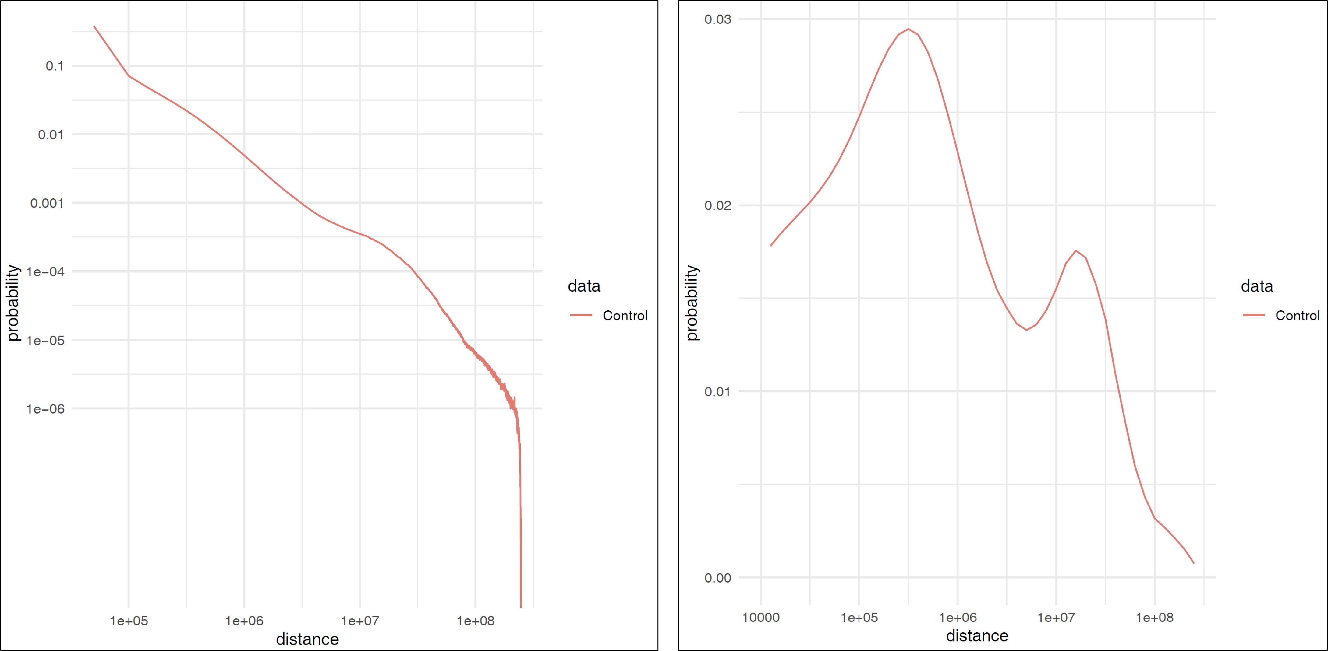
3.5. Plot the fragment distance#
plot_distance_count.sh calcultes the fragment distance and generates a figure (.pdf).
The result is outputted in distance/ directory.
plot_distance_count.sh $cell $odir
Output
distance_vs_count.MAPQ30.pdf … Figure of distance plot
distance_vs_count.MAPQ30.txt … Values for the plot
distance_vs_count.MAPQ30.log.pdf … Figure of distance plot (log scale bins)
distance_vs_count.MAPQ30.log.txt … Values for the plot (log scale bins)
3.6. Make a contact matrix#
makeMatrix_intra.sh takes a .hic file as input and generates the matrices of intra-chromosomal interactions for all chromsomes. The chormosome Y and M are omited.
build=hg38
gt=genometable.$build.txt

cell=Control # siCTCF siRad21
odir=CustardPyResults_Hi-C/Juicer_$build/$cell
hic=$odir/aligned/inter_30.hic
norm=SCALE  # Normalization method (KR|VC|SQRT|VC_SQRT|NONE)
resolution=25000

makeMatrix_intra.sh $norm $odir $hic $resolution $gt
3.7. Calculate insulation scores#
makeInsulationScore.sh takes the observed matrices files generated by makeMatrix_intra.sh as input and calculates the insulation score for all chromsomes. The chormosome Y and M are omited.
build=hg38
gt=genometable.$build.txt

cell=Control # siCTCF siRad21
odir=CustardPyResults_Hi-C/Juicer_$build/$cell
hic=$odir/aligned/inter_30.hic
norm=SCALE  # Normalization method (KR|VC|SQRT|VC_SQRT|NONE)
resolution=25000

makeInsulationScore.sh $norm $odir $resolution $gt
3.8. Call TADs by ArrowHead#
juicer_callTAD.sh uses Juicer ArrowHead to call TADs. By default the resolutions for TADs are 10 kbp, 25 kbp and 50 kbp.
build=hg38
gt=genometable.$build.txt

cell=Control # siCTCF siRad21
odir=CustardPyResults_Hi-C/Juicer_$build/$cell
hic=$odir/aligned/inter_30.hic
norm=SCALE
juicer_callTAD.sh $norm $odir $hic $gt
3.9. Calculate Eigenvector and estimate the compartments A/B#
makeEigen.sh generates eigenvector file (compartment PC1) from a .hic file using HiC1Dmetrics.
The sign (+-) of the value indicating A/B compartments is adjusted by the number of genes.
build=hg38
gt=genometable.$build.txt
gene=refFlat.$build.txt
cell=Control # siCTCF siRad21
odir=CustardPyResults_Hi-C/Juicer_$build/$cell
hic=$odir/aligned/inter_30.hic

norm=SCALE
resolution=25000
ncore=24  # number of cores

makeEigen.sh -p $ncore $norm $odir $hic $resolution $gt $gene
3.10. Call chromatin loops by HICCUPS (GPU required)#
call_HiCCUPS.sh calls loops using Juicer HiCCUPS.
Supply --gpus all for Docker and --nv option for Singularity to activate GPU as follows:
singularity exec --nv custardpy_juicer.sif call_HiCCUPS.sh
docker run --rm -it --gpus all rnakato/custardpy call_HiCCUPS.sh
build=hg38

cell=Control # siCTCF siRad21
odir=CustardPyResults_Hi-C/Juicer_$build/$cell
hic=$odir/aligned/inter_30.hic
norm=SCALE
call_HiCCUPS.sh $norm $odir $hic
3.11. Summarize the statistics of Juicer results#
CustardPy provides a script Juicerstats.sh to summarize the results of Juicer, including mapping reads, number of TADs/loops, etc.
Note that the $odir in this command is the directory of all samples, not each sample as in the other commands.
odir=CustardPyResults_Hi-C/Juicer_$build/
norm=SCALE
Juicerstats.sh $odir $norm
The generated statistics file (Juicerstats.tsv) looks like this:

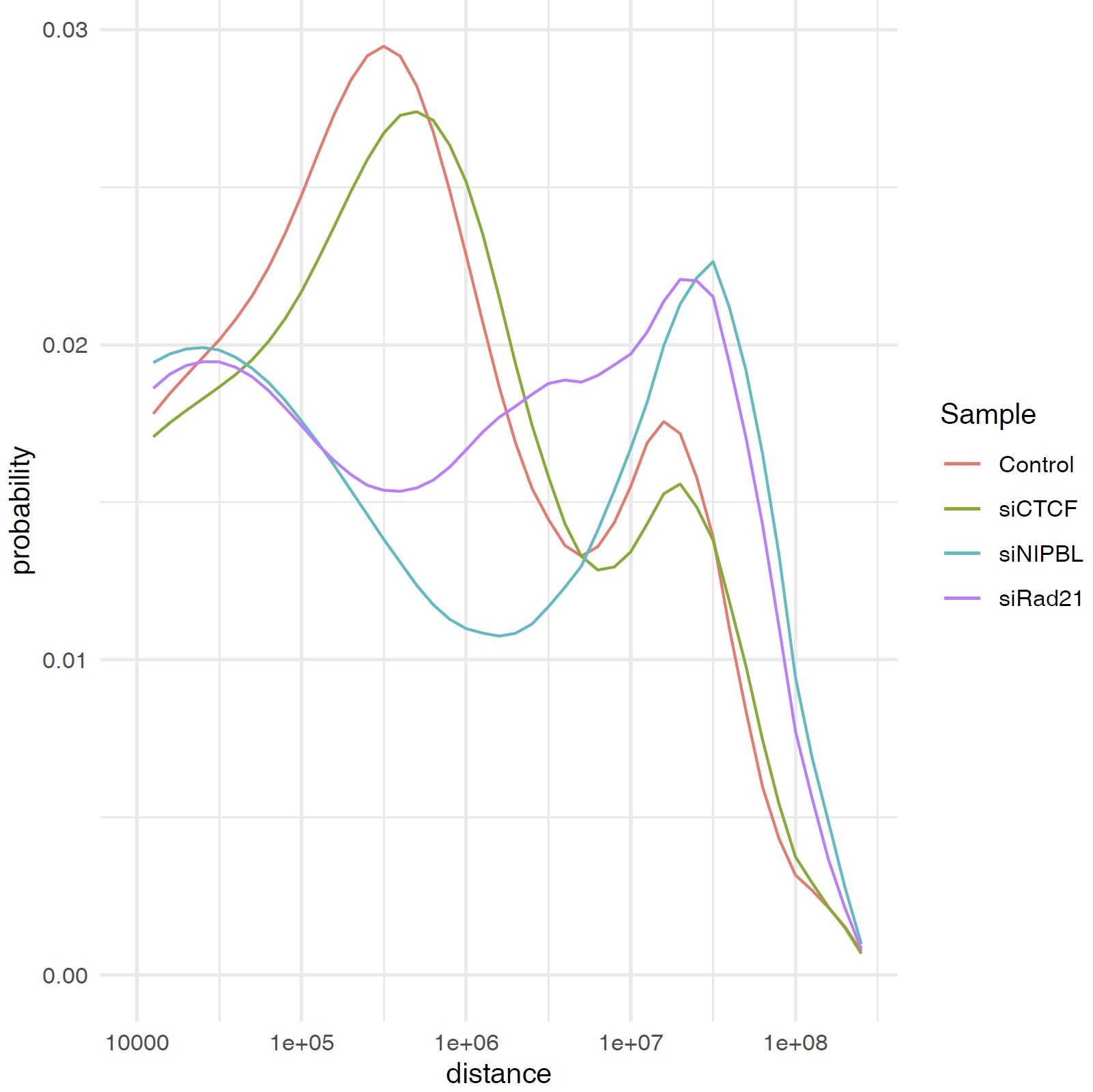
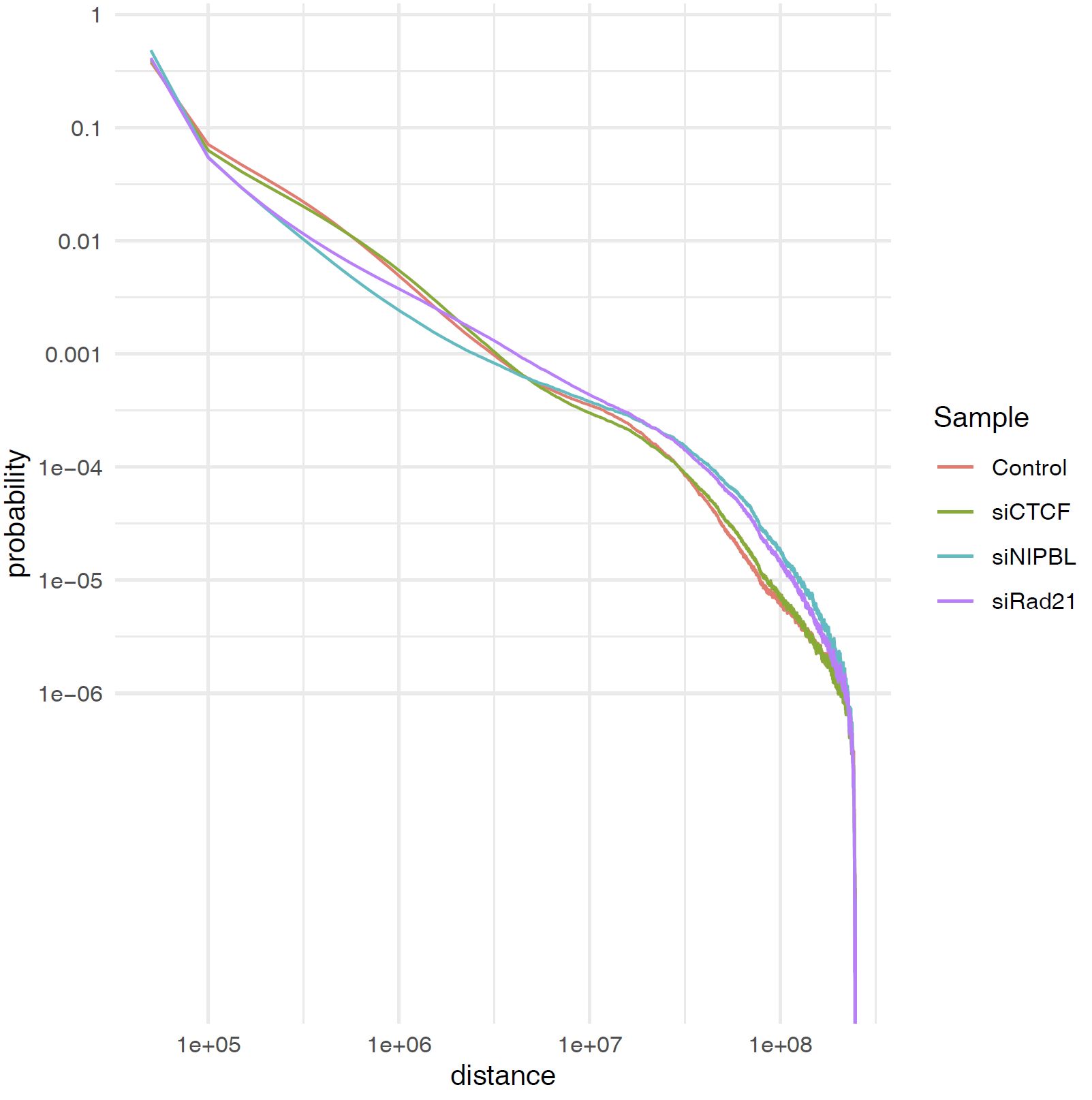
3.12. Plot Contact Distance Distribution for All Samples#
You can use the plot_distance_count_all.R script to plot the contact distance distribution for all samples.
Use the execute_R command to run the R script as follows.
odir=CustardPyResults_Hi-C/Juicer_$build/
execute_R plot_distance_count_all.R $odir $odir/plot_distance_count_all.pdf
execute_R plot_distance_count_all.log.R $odir $odir/plot_distance_count_all.log.pdf
plot_distance_count_all.R and plot_distance_count_all.log.R plot the contact distance distribution in linear and log scale, respectively.
3.13. Plot Contact Distance Distribution for Selected Samples#
When the number of samples is large, the plot of the contact distance distribution for all samples may be difficult to see.
In such a case, you can use the plot_distance_count_multi.R and plot_distance_count_all.log.R scripts to plot the contact distance distribution for selected samples.
odir=CustardPyResults_Hi-C/Juicer_$build/
execute_R plot_distance_count_multi.R $odir/Control $odir/siRad21 $odir/plot_distance_count_multi.pdf
This command plots the contact distance distribution for the control and siRad21 samples. Any number of samples can be specified.