4. Visualization#
This page introduces the commands in CustardPy to plot the 3D visualization.
These commands use the output data generated by custardpy_juicer or custardpy_process_hic.
Here we use the example data used in Step-by-Step Workflow of Hi-C Analysis.
4.1. plotHiCMatrix#
plotHiCMatrix visualizes a contact map as a simple square heatmap. The input data is a dense matrix output from makeMatrix_intra.sh.
The contact level is normalized by the total number of mapped reads for the chromosome.
plotHiCMatrix <matrix> <output name> <start> <end> <title in figure>
Example:
chr=chr20
start=8000000
end=16000000
resolution=25000
norm=SCALE

matrix=CustardPyResults_Hi-C/Juicer_hg38/Control/Matrix/intrachromosomal/$resolution/observed.$norm.$chr.matrix.gz

plotHiCMatrix \
     $matrix \
     ContactMap.Control.$chr.$start-$end.pdf \
     $start $end Control
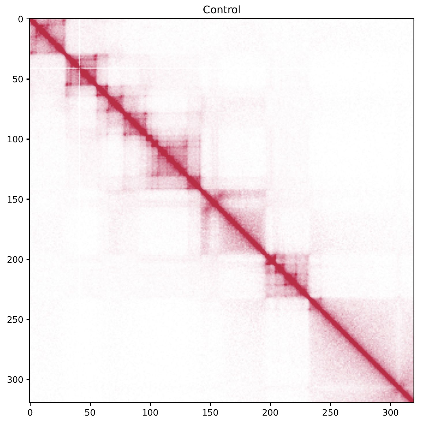
Fig. 4.1 plotHiCMatrix#
4.2. drawSquareMulti#
drawSquareMulti visualizes the contact map of multiple Hi-C samples as triangle heatmaps.
The input data is a dense matrix output from makeMatrix_intra.sh.
Resdir=CustardPyResults_Hi-C/Juicer_hg38
norm=SCALE
resolution=25000
chr=chr20
start=8000000
end=16000000

# linear scale
drawSquareMulti \
  $Resdir/Control:Control \
  $Resdir/siCTCF:siCTCF \
  $Resdir/siRad21:siRad21 \
  -o SquareMulti.$chr \
  -c $chr --start $start --end $end --type $norm -r $resolution
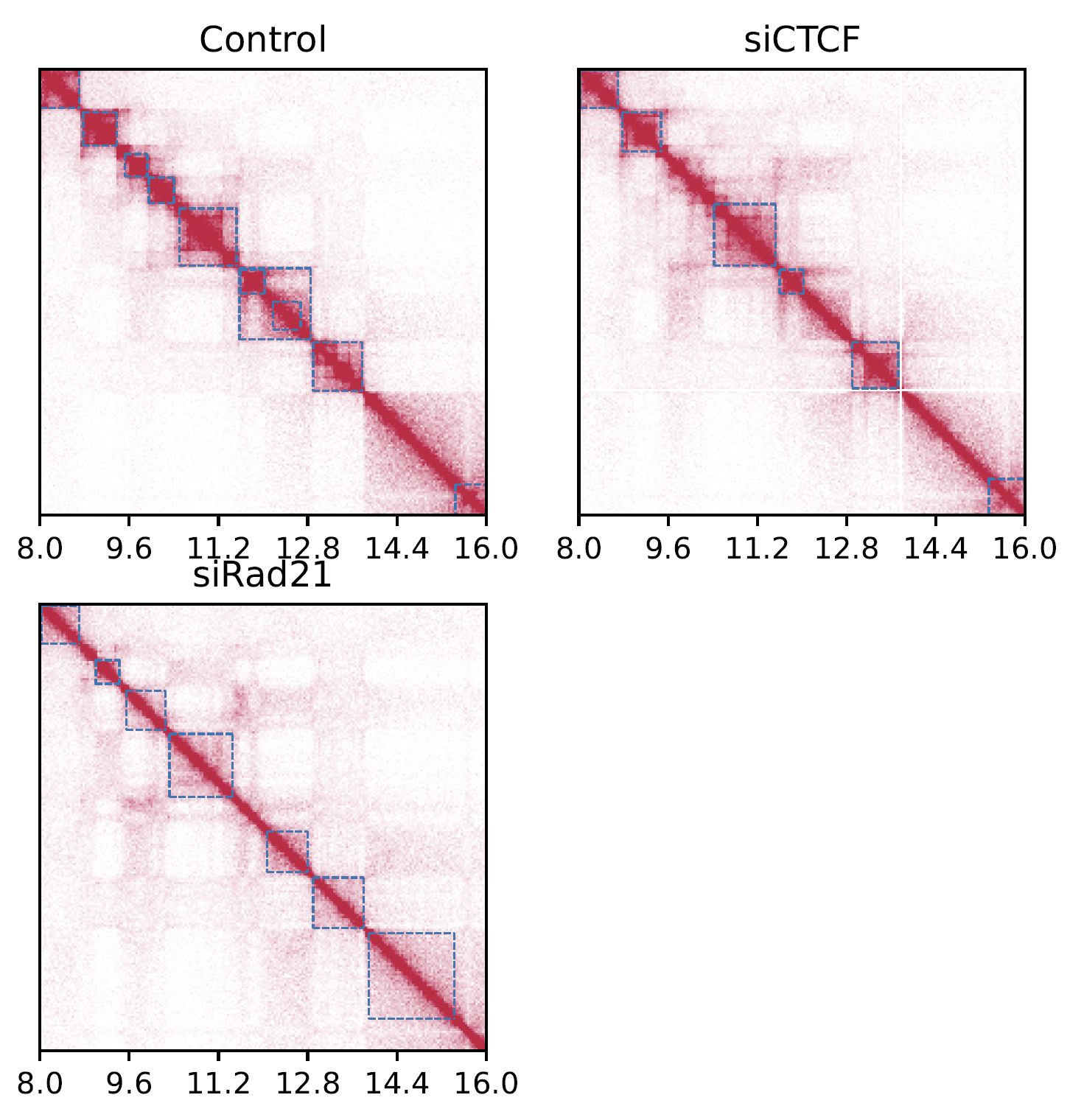
Fig. 4.2 SquareMulti#
The dashed squares indicate TADs.
Add --log option to visualize a log-scale heatmap.
# log scale
drawSquareMulti \
  $Resdir/Control:Control \
  $Resdir/siCTCF:siCTCF \
  $Resdir/siRad21:siRad21 \
  -o SquareMulti.$chr \
  -c $chr --start $start --end $end \
  --type $norm -r $resolution --log
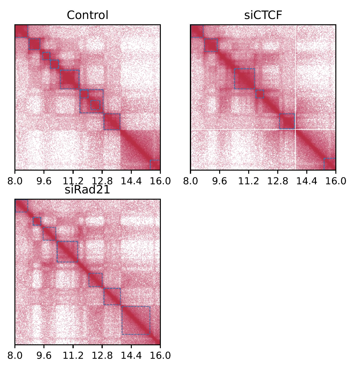
Fig. 4.3 SquareMulti (log scale)#
4.3. drawSquareRatioMulti#
drawSquareRatioMulti visualizes a relative contact frequency (log scale) of 2nd to the last samples against the first sample.
The input data is a dense matrix output from makeMatrix_intra.sh.
Resdir=CustardPyResults_Hi-C/Juicer_hg38
norm=SCALE
resolution=25000
chr=chr20
start=8000000
end=16000000

drawSquareRatioMulti \
     $Resdir/Control:Control \
     $Resdir/siCTCF:siCTCF \
     $Resdir/siRad21:siRad21 \
     -o SquareRatioMulti.$chr \
     -c $chr --start $start --end $end --type $norm -r $resolution
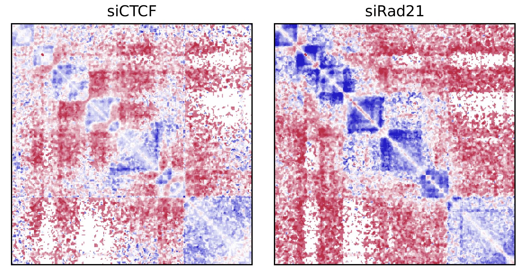
Fig. 4.4 drawSquareRatioMulti#
This figure shows the relative contact frequency of 2nd (siCTCF) and 3rd (siRad21) against 1st (Control).
4.4. drawSquarePair#
drawSquarePair shows two samples in a single square heatmap.
The first and second samples are visualzed in the upper and bottom triagles, respectively.
Resdir=CustardPyResults_Hi-C/Juicer_hg38
norm=SCALE
resolution=25000
chr=chr20
start=8000000
end=16000000

drawSquarePair \
     $Resdir/Control/Matrix/intrachromosomal/$resolution/observed.$norm.$chr.matrix.gz:Control \
     $Resdir/siRad21/Matrix/intrachromosomal/$resolution/observed.$norm.$chr.matrix.gz:siRad21 \
     -o SquarePair.$chr --start $start --end $end -r $resolution
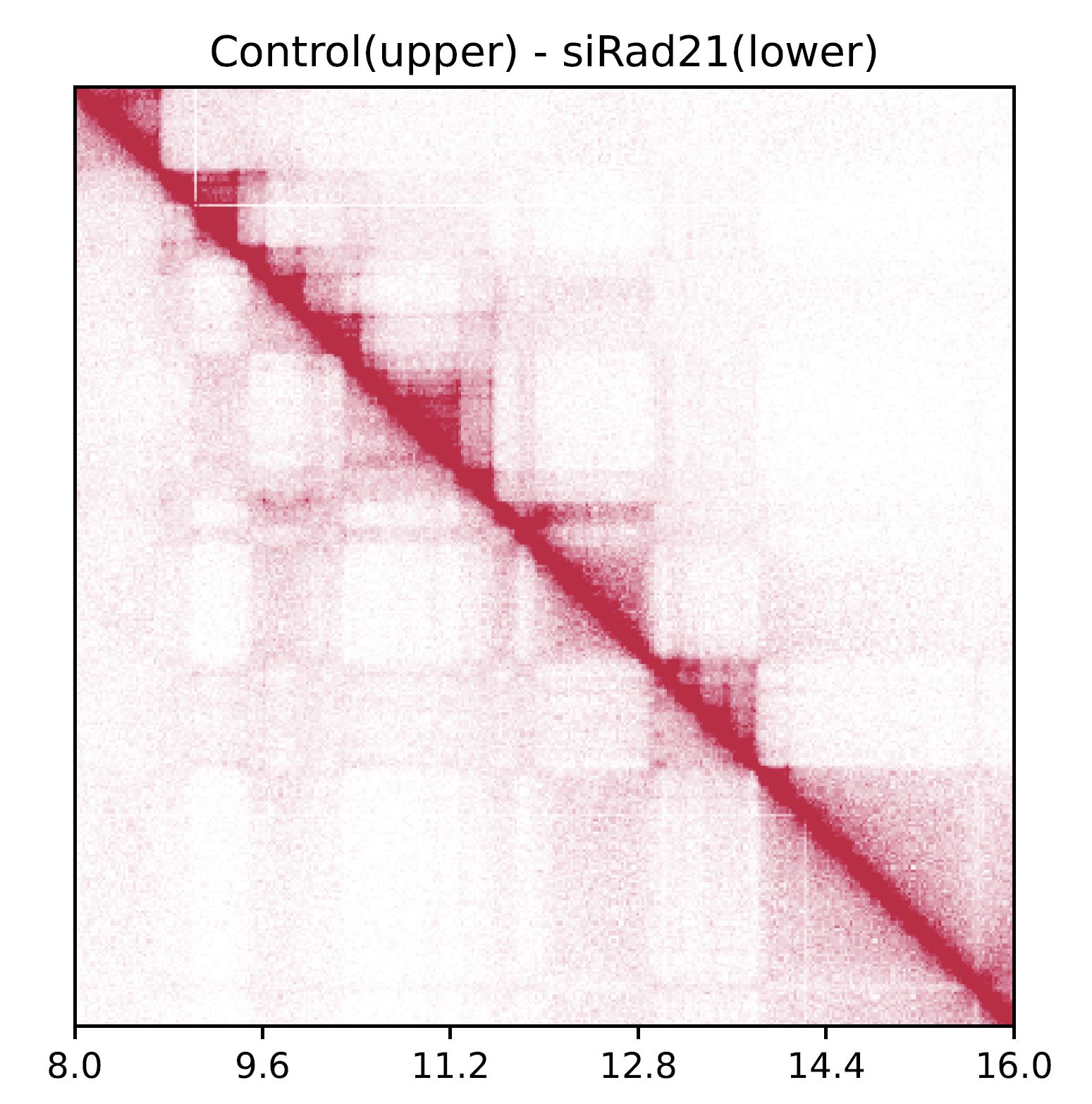
Fig. 4.5 drawSquarePair#
The command visualizes Control and siRad21 in the upper and bottom triagles, respectively.
4.5. drawSquareRatioPair#
Similar to drawSquarePair, drawSquareRatioPair shows the relative contact map of two sample pairs in a single square heatmap.
This command visualize the log-scale frequency of sample2/sample1 and sample4/sample3 in the upper and bottom triagles, respectively.
Resdir=CustardPyResults_Hi-C/Juicer_hg38
norm=SCALE
resolution=25000
chr=chr20
start=8000000
end=16000000

drawSquareRatioPair \
     $Resdir/Control/Matrix/intrachromosomal/$resolution/observed.$norm.$chr.matrix.gz:Control \
     $Resdir/siRad21/Matrix/intrachromosomal/$resolution/observed.$norm.$chr.matrix.gz:siRad21 \
     $Resdir/Control/Matrix/intrachromosomal/$resolution/observed.$norm.$chr.matrix.gz:Control \
     $Resdir/siCTCF/Matrix/intrachromosomal/$resolution/observed.$norm.$chr.matrix.gz:siCTCF \
     -o drawSquareRatioPair.$chr --start $start --end $end -r $resolution
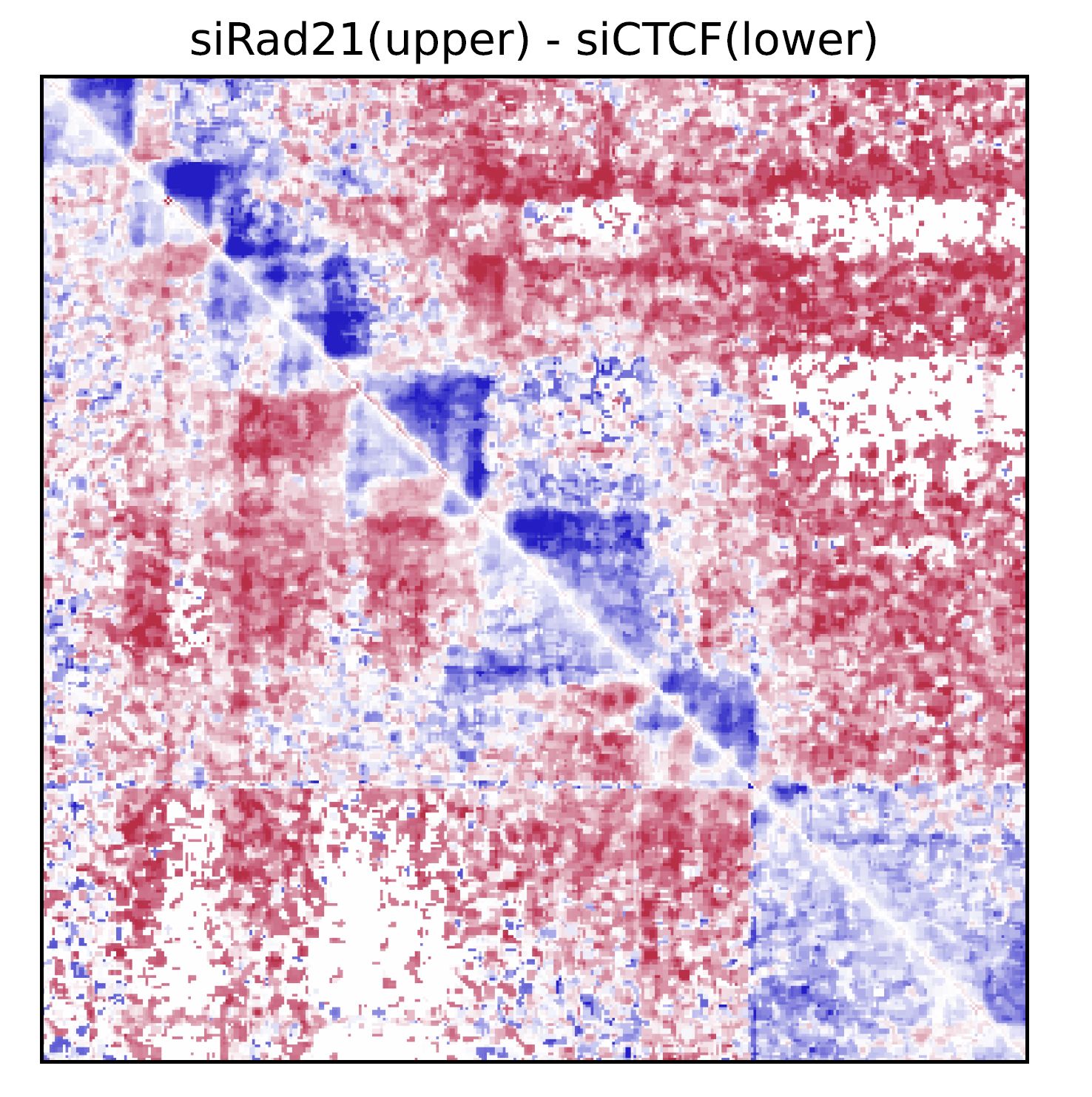
Fig. 4.6 drawSquareRatioPair#
In this case, siRad21/Control and siCTCF/Control are visualized in the upper and bottom triagles, respectively.
4.6. drawTriangleMulti#
drawTriangleMulti visualizes the contact map of multiple Hi-C samples as triangle heatmaps.
The input data is a dense matrix output from makeMatrix_intra.sh.
Resdir=CustardPyResults_Hi-C/Juicer_hg38
norm=SCALE
resolution=25000
chr=chr20
start=8000000
end=16000000

drawTriangleMulti \
     $Resdir/Control:Control \
     $Resdir/siCTCF:siCTCF \
     $Resdir/siRad21:siRad21 \
     -o TriangleMulti.$chr \
     -c $chr --start $start --end $end --type $norm -d 5000000 -r $resolution
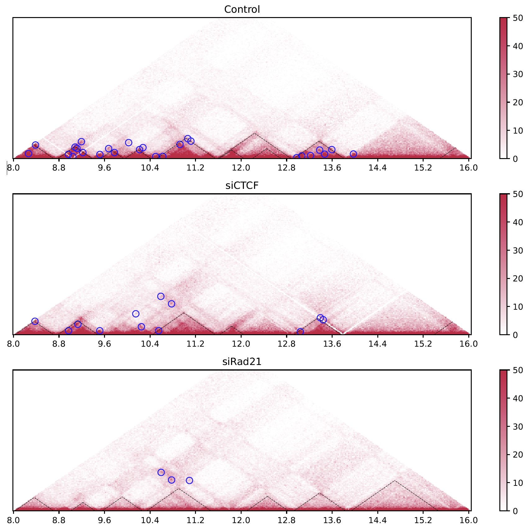
Fig. 4.7 drawTriangleMulti#
The black dashed lines and blue circles indicate TADs and loops, respectively.
4.7. drawTrianglePair#
drawTrianglePair visualizes a contact map of the first and second sample in upper and lower triangles, respectively.
Resdir=CustardPyResults_Hi-C/Juicer_hg38
norm=SCALE
resolution=25000
chr=chr20
start=8000000
end=16000000

drawTrianglePair \
     $Resdir/Control:Control \
     $Resdir/siRad21:siRad21 \
     -o TrianglePair.$chr \
     -c $chr --start $start --end $end --type $norm -d 5000000 -r $resolution
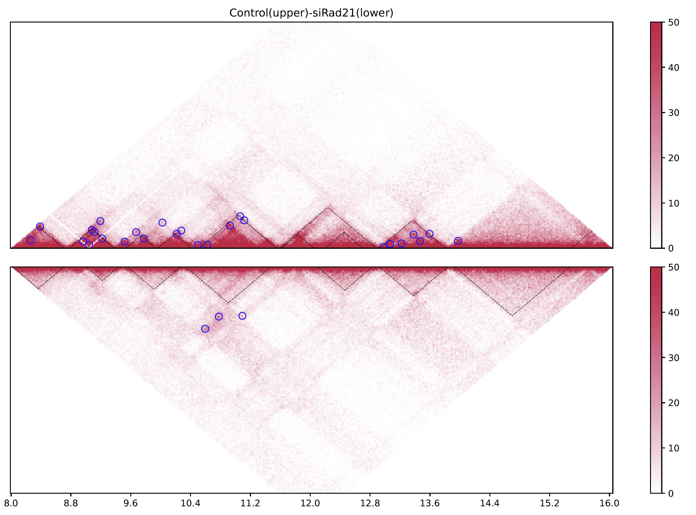
Fig. 4.8 drawTrianglePair#
The black dashed lines and blue circles indicate TADs and loops, respectively.
4.8. plotHiCfeature#
plotHiCfeature can visualize various features values of chromatin folding for multiple samples.
plotHiCfeature [-h] [-o OUTPUT] [-c CHR] [--type TYPE]
               [--distance DISTANCE] [-r RESOLUTION] [-s START]
               [-e END] [--multi] [--multidiff] [--compartment] [--di]
               [--drf] [--drf_right] [--drf_left]
               [--triangle_ratio_multi] [-d VIZDISTANCEMAX] [--v4c]
               [--vmax VMAX] [--vmin VMIN] [--vmax_ratio VMAX_RATIO]
               [--vmin_ratio VMIN_RATIO] [--anchor ANCHOR]
               [--xsize XSIZE]
               [input [input ...]]

positional arguments:
     input                 <Input directory>:<label>

optional arguments:
     -h, --help            show this help message and exit
     -o OUTPUT, --output OUTPUT
                         Output prefix
     -c CHR, --chr CHR     chromosome
     --type TYPE           normalize type (default: SCALE)
     --distance DISTANCE   distance for DI (default: 500000)
     -r RESOLUTION, --resolution RESOLUTION
                         resolution (default: 25000)
     -s START, --start START
                         start bp (default: 0)
     -e END, --end END     end bp (default: 1000000)
     --multi               plot MultiInsulation Score
     --multidiff           plot differential MultiInsulation Score
     --compartment         plot Compartment (eigen)
     --di                  plot Directionaly Index
     --drf                 plot Directional Relative Frequency
     --drf_right           (with --drf) plot DirectionalRelativeFreq (Right)
     --drf_left            (with --drf) plot DirectionalRelativeFreq (Left)
     --triangle_ratio_multi
                         plot Triangle ratio multi
     -d VIZDISTANCEMAX, --vizdistancemax VIZDISTANCEMAX
                         max distance in heatmap
     --v4c                 plot virtual 4C from Hi-C data
     --vmax VMAX           max value of color bar (default: 50)
     --vmin VMIN           min value of color bar (default: 0)
     --vmax_ratio VMAX_RATIO
                         max value of color bar for logratio (default: 1)
     --vmin_ratio VMIN_RATIO
                         min value of color bar for logratio (default: -1)
     --anchor ANCHOR       (for --v4c) anchor point
     --xsize XSIZE         xsize for figure (default: max(length/2M, 10))
Inputshould be “<sample directory>:<label>”.<sample directory>is the output directory bycustardpy_juicer.<label>is the label used in the figure.
In default,
plotHiCfeatureuses a 25-kbp bin matrix. Supply-roption to change the resolution.typeis the normalization type defined by Juicer (SCALE/KR/VC_SQRT/NONE).
4.8.1. Insulation score#
By default, plotHiCfeature outputs a single insulation score (500 kbp distance).
Resdir=CustardPyResults_Hi-C/Juicer_hg38
norm=SCALE
resolution=25000
chr=chr20
start=8000000
end=16000000

plotHiCfeature \
     $Resdir/Control:Control \
     $Resdir/siCTCF:siCTCF \
     $Resdir/siRad21:siRad21 \
     -c $chr --start $start --end $end -r $resolution \
     --type $norm -d 5000000 \
     -o IS.$chr.$start-$end
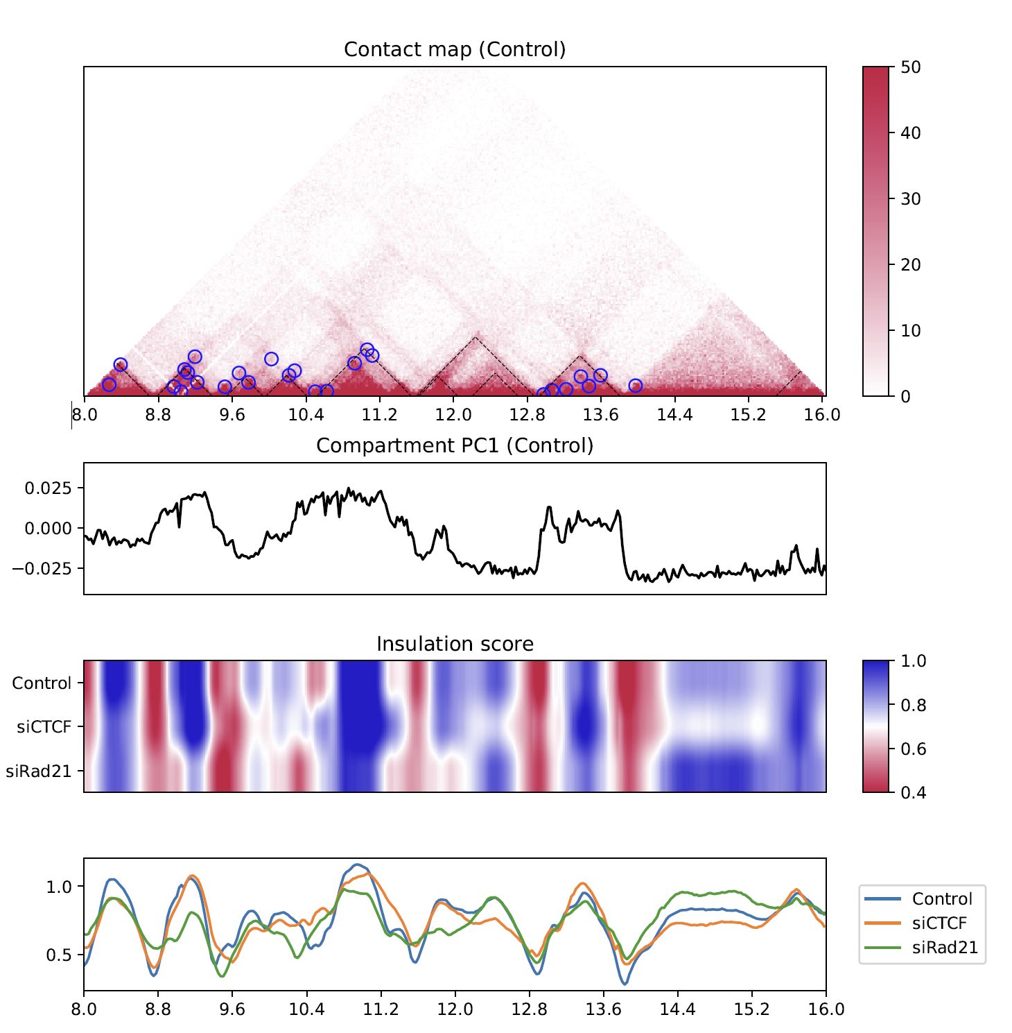
Fig. 4.9 Insulation score#
plotHiCfeature always draws compartment PC1 (line plot in the second row) to roughly estimate compartments A and B.
The third and fourth rows are the heatmap and line plot for the feature value specified (insulation score in this case).
4.8.2. Multi-insulation score#
plotHiCfeature can also calculate a “multi-scale insulation score” [Crane et al., Nature, 2015] by supplying --multi option.
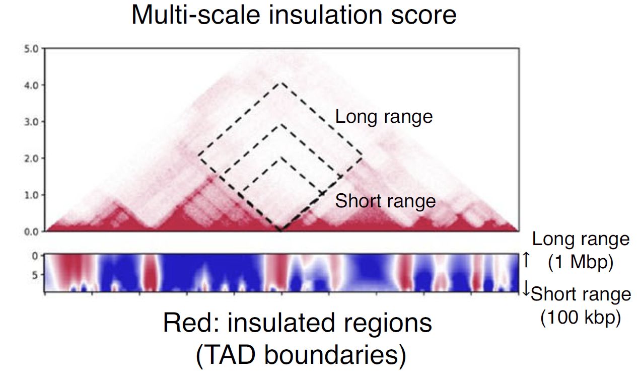
Fig. 4.10 Schematic illustration of multi-insulation score#
Red regions in the heatmap indicate the insulated regions (TAD boundary-like). The lower and upper sides of the heatmap are 100 kbp to 1 Mbp distances, respectively.
Resdir=CustardPyResults_Hi-C/Juicer_hg38
norm=SCALE
resolution=25000
chr=chr20
start=8000000
end=16000000

plotHiCfeature \
     $Resdir/Control:Control \
     $Resdir/siCTCF:siCTCF \
     $Resdir/siRad21:siRad21 \
     -c $chr --start $start --end $end -r $resolution \
     --multi --type $norm -d 5000000 \
     -o MultiIS.$chr.$start-$end
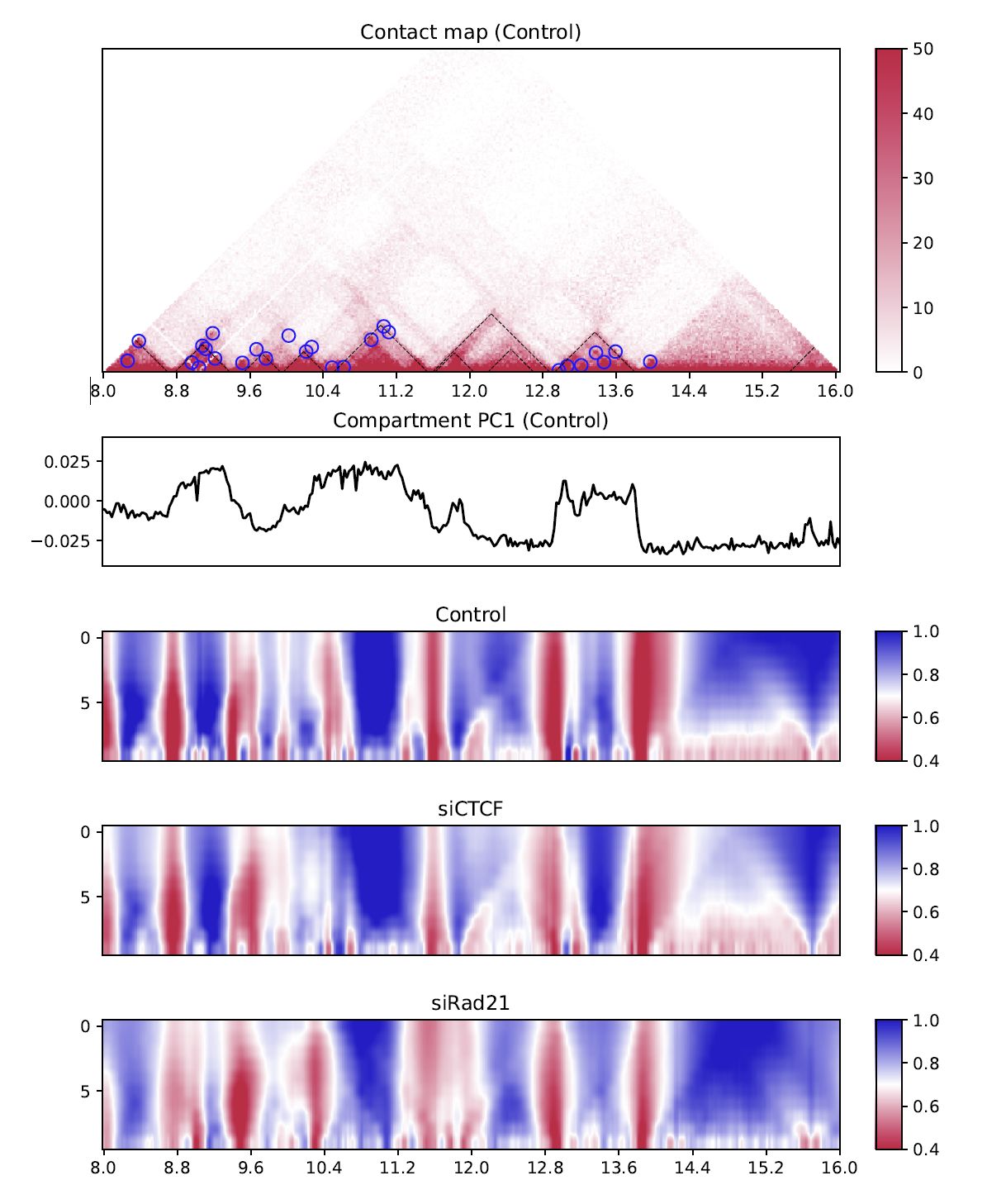
Fig. 4.11 Multi-insulation score#
4.8.3. Differential multi-insulation score#
To directory investigate the difference of multi-insulation score, we provide differential multi-insulation score by --multidiff option.
Resdir=CustardPyResults_Hi-C/Juicer_hg38
norm=SCALE
resolution=25000
chr=chr20
start=8000000
end=16000000

plotHiCfeature \
     $Resdir/Control:Control \
     $Resdir/siCTCF:siCTCF \
     $Resdir/siRad21:siRad21 \
     -c $chr --start $start --end $end -r $resolution \
     --multidiff --type $norm -d 5000000 \
     -o MultiISdiff.$chr.$start-$end
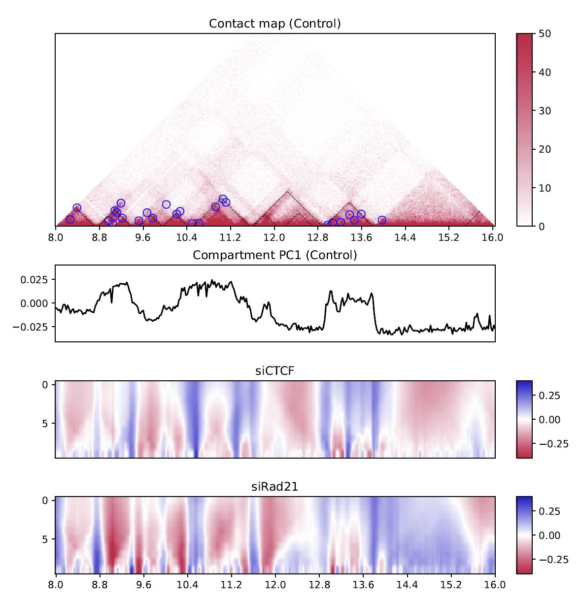
Fig. 4.12 Differential multi-insulation score#
The heatmap shows the difference against the first sample (siCTCF - Control and siRad21 - Control in this case).
4.8.4. Compartment PC1#
While the line plot in the second row shows the PC1 value of the first sample,
plotHiCfeature --compartment visualizes the PC1 values for multiple samples.
This plot can be used to explore compartment switching.
Resdir=CustardPyResults_Hi-C/Juicer_hg38
norm=SCALE
resolution=25000
chr=chr20
start=8000000
end=16000000

plotHiCfeature \
     $Resdir/Control:Control \
     $Resdir/siCTCF:siCTCF \
     $Resdir/siRad21:siRad21 \
     -c $chr --start $start --end $end -r $resolution \
     --compartment --type $norm -d 5000000 \
     -o Compartment.$chr.$start-$end
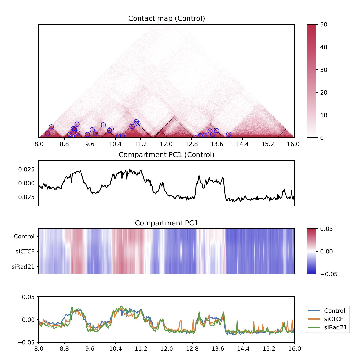
Fig. 4.13 Compartment PC1#
4.8.5. Directionality index#
The directionality index identifies TAD boundaries by capturing the bias in contact frequency up- and downstream of a TAD [Dixon et al., Nature, 2012]. The “left side” and “right side” of a TAD are likely to have positve and negative values, respectively.
Resdir=CustardPyResults_Hi-C/Juicer_hg38
norm=SCALE
resolution=25000
chr=chr20
start=8000000
end=16000000

plotHiCfeature \
     $Resdir/Control:Control \
     $Resdir/siCTCF:siCTCF \
     $Resdir/siRad21:siRad21 \
     -c $chr --start $start --end $end -r $resolution \
     --di --type $norm -d 5000000 \
     -o DI.$chr.$start-$end
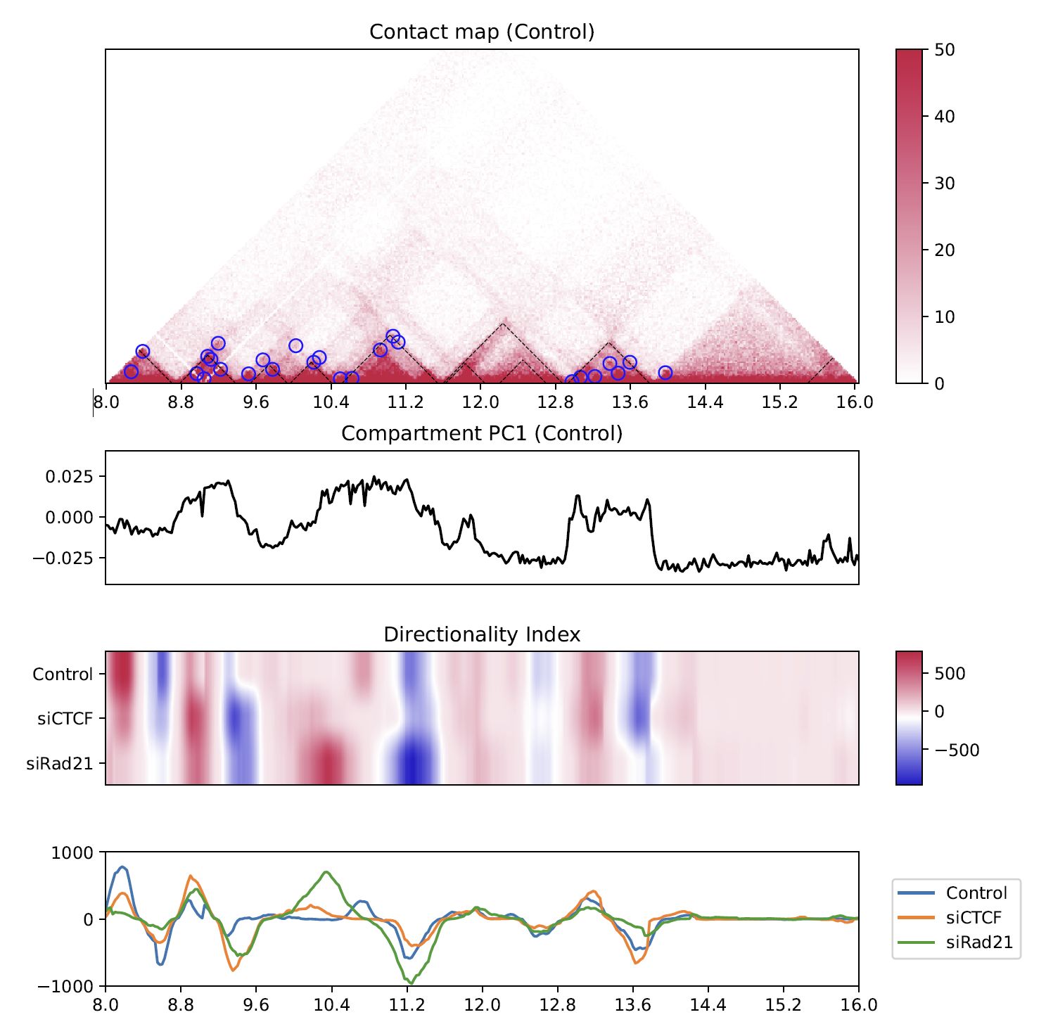
Fig. 4.14 Directionality index#
4.8.6. Directional relative frequency#
Directional relative frequency (DRF) is a score that our group previously proposed [Nakato et al, Nature Communications, 2023]. This score estimates the inconsistency of relative contact frequence (log scale) between the left side (3′) and right side (5′).
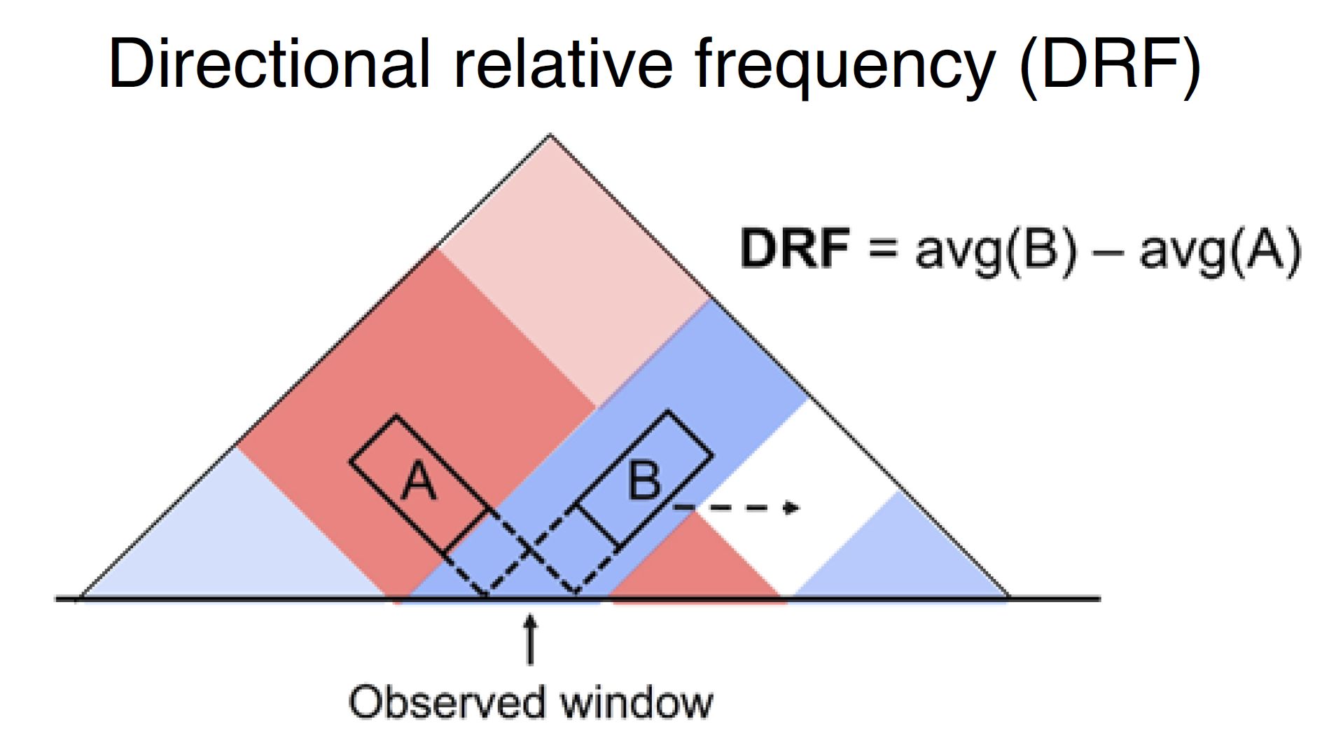
Fig. 4.15 Schematic illustration of directional relative frequency#
Resdir=CustardPyResults_Hi-C/Juicer_hg38
norm=SCALE
resolution=25000
chr=chr20
start=8000000
end=16000000

plotHiCfeature \
     $Resdir/Control:Control \
     $Resdir/siCTCF:siCTCF \
     $Resdir/siRad21:siRad21 \
     -c $chr --start $start --end $end -r $resolution \
     --drf --type $norm -d 5000000 \
     -o DRF.$chr.$start-$end
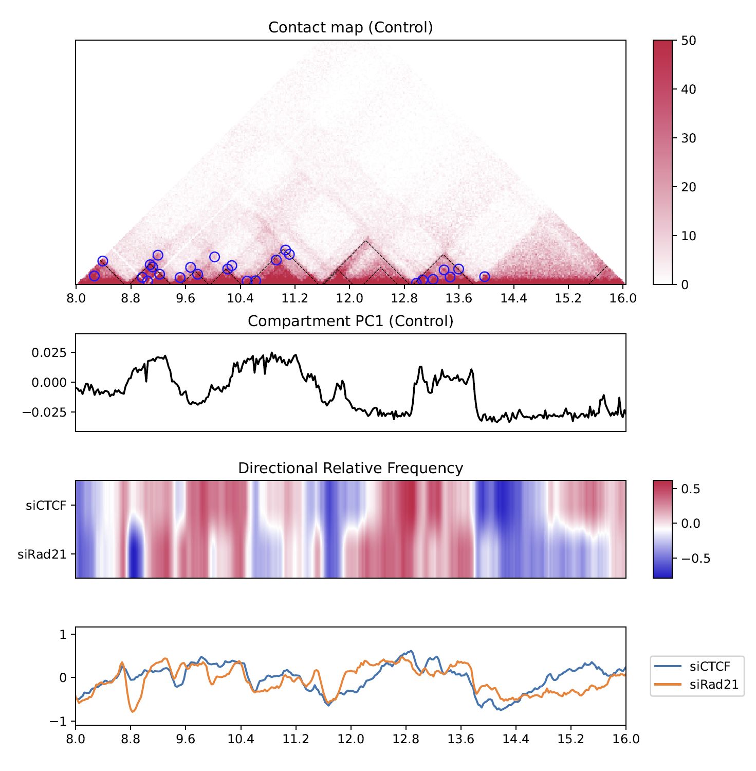
Fig. 4.16 Directional relative frequency#
4.8.7. drawTriangleRatioMulti#
--triangle_ratio_multi visualizes a relative contact frequency (log scale) of 2nd to the last samples against the first sample. Directional relative frequency is also shown.
Resdir=CustardPyResults_Hi-C/Juicer_hg38
norm=SCALE
resolution=25000
chr=chr20
start=8000000
end=16000000

plotHiCfeature \
     $Resdir/Control:Control \
     $Resdir/siCTCF:siCTCF \
     $Resdir/siRad21:siRad21 \
     -o TriangleRatioMulti.$chr \
     -c $chr --start $start --end $end -r $resolution \
     --triangle_ratio_multi --type $norm -d 5000000
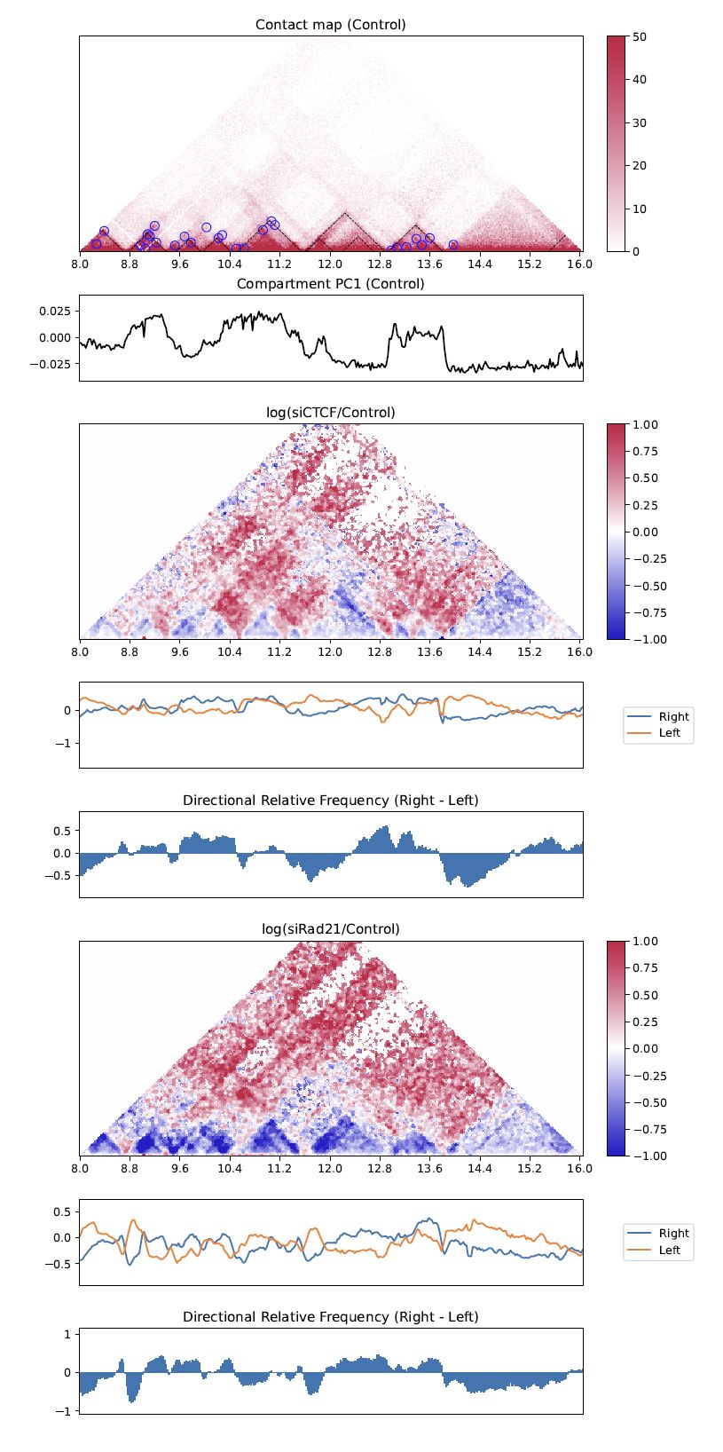
Fig. 4.17 TriangleRatioMulti#
“Right” and “left” shown as blue and orange line plots in the second row indicate the “B” and “A” in Fig. 4.15.
4.8.8. Output the logfold change matrices#
--triangle_ratio_multi has an option --output_logfc_matrix to output the logfold change matrices used for the visualization.
This command is useful if you want to do a downstream analysis using the matrices.
Resdir=CustardPyResults_Hi-C/Juicer_hg38
norm=SCALE
resolution=25000
chr=chr20
start=8000000
end=16000000

plotHiCfeature \
     $Resdir/Control:Control \
     $Resdir/siCTCF:siCTCF \
     $Resdir/siRad21:siRad21 \
     -o TriangleRatioMulti.$chr \
     -c $chr --start $start --end $end -r $resolution \
     --triangle_ratio_multi --type $norm -d 5000000 \
     --output_logfc_matrix
4.8.9. Virtual 4C#
Virtual 4C visualizes a 4C-like plot (interation from the anchor site) using Hi-C data.
Use --anchor option to specify the anchor site.
Resdir=CustardPyResults_Hi-C/Juicer_hg38
norm=SCALE
resolution=25000
chr=chr20
start=8000000
end=16000000

plotHiCfeature \
     $Resdir/Control:Control \
     $Resdir/siCTCF:siCTCF \
     $Resdir/siRad21:siRad21 \
     -o virtual4C.$chr \
     -c $chr --start $start --end $end -r $resolution \
     --v4c --anchor 10400000 --vmax 100 --type $norm
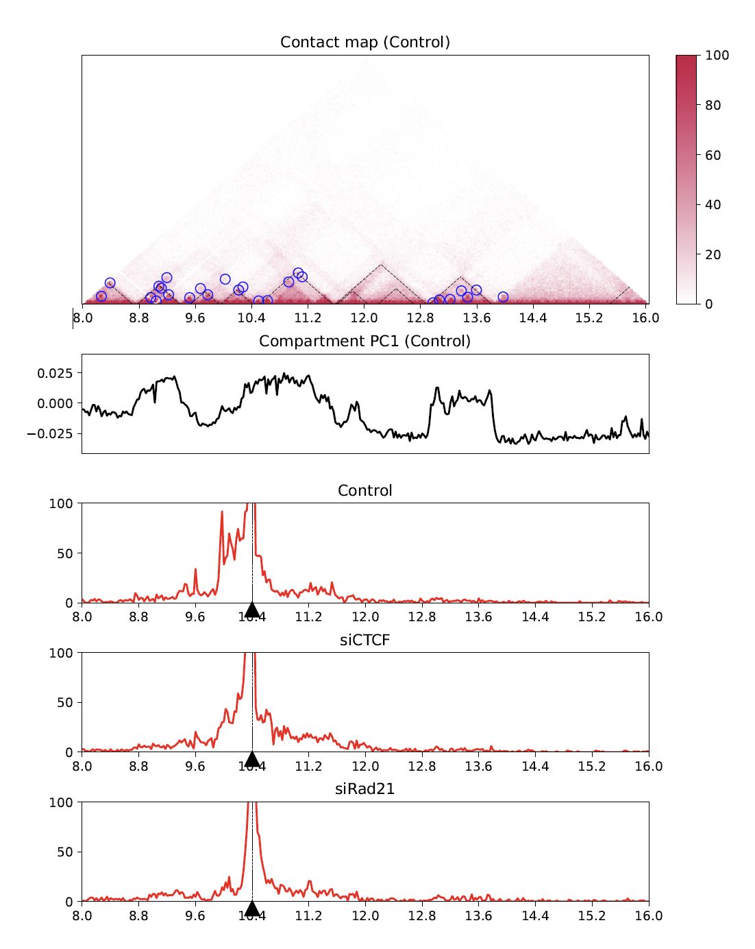
Fig. 4.18 Virtual 4C#
4.9. plotCompartmentGenome#
Plot a PC1 value of multiple samples for the whole genome.
Resdir=CustardPyResults_Hi-C/Juicer_hg38
norm=SCALE
resolution=25000
chr=chr20
start=8000000
end=16000000

plotCompartmentGenome
     $Resdir/Control:Control \
     $Resdir/siCTCF:siCTCF \
     $Resdir/siRad21:siRad21 \
     -o CompartmentGenome -r 25000 --type VC_SQRT
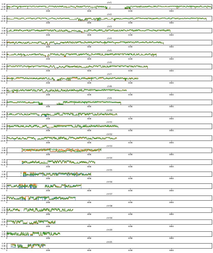
Fig. 4.19 plotCompartmentGenome#
4.10. plotInsulationScore#
Plot a line graph of insulation score. The input data is a dense matrix output from makeMatrix_intra.sh.
plotInsulationScore [-h] [--num4norm NUM4NORM] [--distance DISTANCE]
                            [--sizex SIZEX] [--sizey SIZEY]
                            matrix output resolution
Example:
   plotInsulationScore WT/intrachromosomal/25000/observed.KR.chr7.matrix.gz InsulationScore_WT.chr7.png 25000
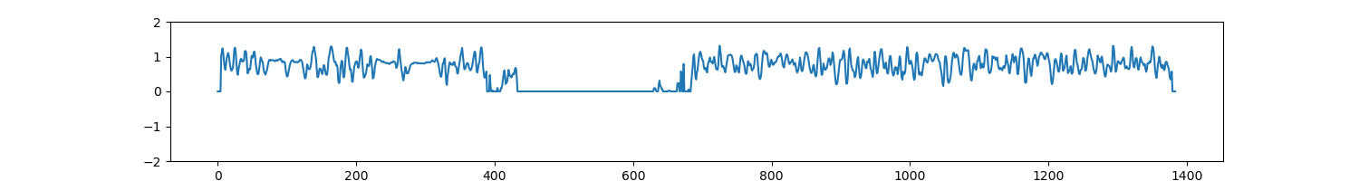
Fig. 4.20 InsulationScore#
4.11. plotMultiScaleInsulationScore#
Plot multi-scale insulation scores from Juicer matrix.
plotMultiScaleInsulationScore [-h] [--num4norm NUM4NORM]
                              [--sizex SIZEX] [--sizey SIZEY]
                              matrix output resolution
Example:
   plotInsulationScore WT/intrachromosomal/25000/observed.KR.chr7.matrix.gz MultiInsulationScore_WT.chr7.png 25000

Fig. 4.21 Multi-Insulation Score (chr7)#